---
title: "Diffusion Models"
subtitle: "Forward corruption, learned denoising, sampling, and conditioning"
---
## Chapter orientation
Diffusion models generate an image by learning to reverse a controlled corruption process. Training starts from a data image, adds noise at a randomly chosen time step, and trains a network to predict the noise or a related denoising target. Sampling starts from noise and applies the learned reverse process repeatedly. This makes the number of denoising steps, the noise schedule, and conditioning interface part of the model's behaviour [@ho2020ddpm].
::: {.concept-box .concept-core #concept-diffusion data-term="Diffusion model" data-domain="Modern AI systems"}
**Diffusion model.** A generative model trained to reverse a declared corruption process. Training estimates a denoising relation; sampling repeatedly applies that relation under a schedule and any conditioning or guidance policy.
:::
## Level 1 - From noise to an image
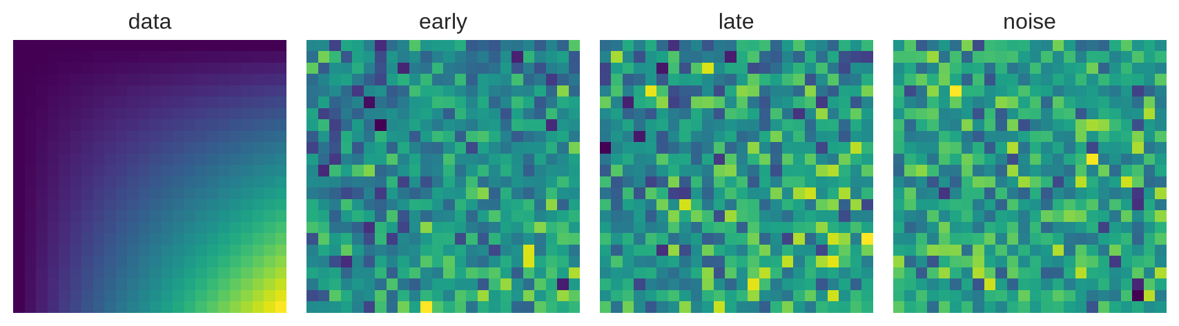
The forward process gradually destroys image structure. The reverse model receives a noisy image and its time step, then predicts how to remove some of that noise. One prediction does not usually recover a complete image; generation is an iterative sequence of denoising decisions.
```{python}
#| label: fig-forward-diffusion
#| fig-cap: "The forward process adds progressively more noise to a data image until visual structure is largely obscured."
#| fig-alt: "Four small image grids run from a structured pattern to increasingly noisy arrays."
import numpy as np
import matplotlib.pyplot as plt
plt.style.use("seaborn-v0_8-whitegrid")
rng=np.random.default_rng(4); x0=np.outer(np.linspace(0,1,24),np.linspace(0,1,24))
fig,axs=plt.subplots(1,4,figsize=(9,2.5))
for ax,a,title in zip(axs,[0,.25,.6,1],["data","early","late","noise"]):
 ax.imshow(np.sqrt(1-a)*x0+np.sqrt(a)*rng.normal(size=x0.shape),cmap="viridis");ax.set_title(title);ax.axis("off")
plt.tight_layout();plt.show()
```
```{python}
x_t=np.array([.3,-.1,.7]); predicted_noise=np.array([.1,-.2,.2]); print(x_t-predicted_noise)
```
## Level 2 - Schedule, denoiser, and sampling
### The schedule defines what the denoiser sees
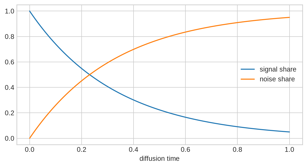
At time (t), a schedule determines the mixture of original signal and Gaussian noise. A common representation is (x_t=\sqrt{\bar\alpha_t}x_0+\sqrt{1-\bar\alpha_t}\epsilon). The denoiser must therefore use both (x_t) and (t): the same noisy value can require different corrections at different noise levels. A schedule that adds noise too quickly can remove useful training signal; a schedule that changes slowly can require more steps.
```{python}
#| label: fig-noise-schedule
#| fig-cap: "A noise schedule controls the declining signal share and rising noise share across diffusion time steps."
#| fig-alt: "Two curves show signal decreasing and noise increasing from time zero to the final diffusion step."
t=np.linspace(0,1,100); signal=np.exp(-3*t); fig,ax=plt.subplots(figsize=(6.5,3.6));ax.plot(t,signal,label="signal share");ax.plot(t,1-signal,label="noise share");ax.legend();ax.set_xlabel("diffusion time");plt.tight_layout();plt.show()
```
### Sampling is a compute-quality trade-off
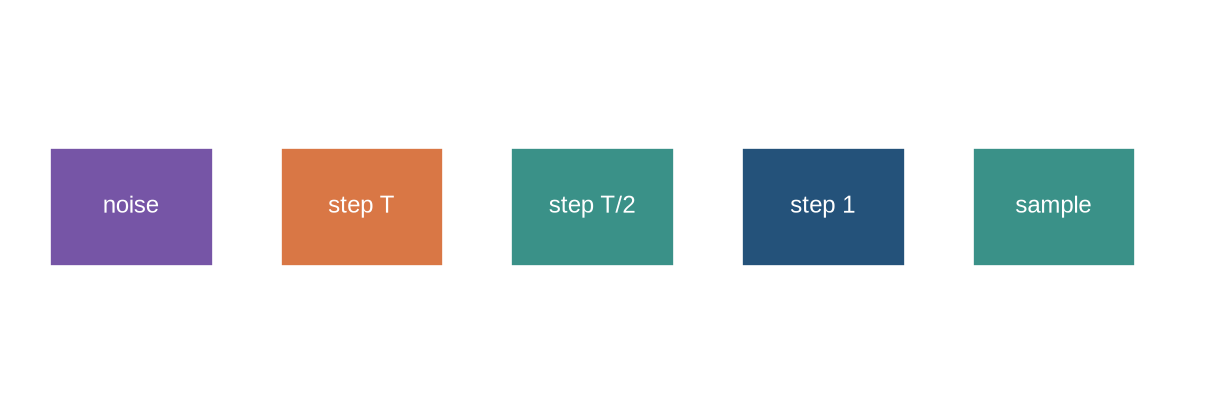
The reverse chain is expensive because it calls the denoiser repeatedly. Faster samplers can use fewer steps but must be evaluated at a matched conditioning, resolution, seed policy, and quality measure. DDIM retains the training objective while permitting faster deterministic or partially stochastic sampling trajectories [@song2020ddim].
The training target and the sampling rule must be kept distinct. Training commonly selects one time step per image and minimises error in a predicted noise term; sampling applies a sequence of model calls whose errors can accumulate. A model can have a low average training loss while producing poor samples at a particular guidance scale, resolution, or condition. Report the time-step distribution, target parameterisation, schedule, sampler, step count, and randomisation policy together.
The basic training calculation makes this distinction concrete. Draw a clean training image (x_0), a noise vector (epsilon), and a time step (t). Use the schedule to form (x_t), then provide (x_t) and a representation of (t) to the denoiser. If the model predicts \(\hat\epsilon_\theta(x_t,t)\), a common loss is the mean squared difference between \(\hat\epsilon\) and the sampled \(\epsilon\). The target is known because the training procedure created the corruption. The model is not shown a target clean image at every reverse sampling step; it must generalise its learned correction from many noisy examples.
The reverse update uses the predicted noise together with coefficients implied by the schedule. Its purpose is to move the current state toward a less noisy distribution while retaining an appropriate amount of uncertainty. An implementation therefore has at least four linked contracts: the forward schedule used to create training inputs, the time representation, the denoiser target, and the reverse solver. Changing one while retaining the others can make a checkpoint or a reported sample comparison invalid.
```{python}
# A toy single-step noise-prediction loss: real image models use tensors and many time steps.
rng=np.random.default_rng(7)
x0=np.array([.2,.7,-.1]); epsilon=rng.normal(size=3); alpha_bar=.64
x_t=np.sqrt(alpha_bar)*x0+np.sqrt(1-alpha_bar)*epsilon
predicted=np.array([.1,-.2,.3])
print("noise loss:",np.mean((predicted-epsilon)**2))
```
Classifier-free guidance illustrates the trade-off. It combines conditional and unconditional denoising predictions to increase the influence of a condition. Raising its scale can improve apparent prompt adherence while producing artefacts or reducing diversity. It is therefore a generation control to evaluate, not a free improvement to attach to a model result.
### Reverse solvers define the sampling trajectory
The schedule supplies a family of noisy distributions; the solver determines how the model traverses them at generation time. A stochastic solver introduces fresh random variation at reverse steps. A deterministic solver can map a fixed initial noise and condition to a repeatable trajectory. Reduced-step solvers select a subset of training-time noise levels or approximate a longer trajectory. These alternatives may have the same denoiser checkpoint but different latency, diversity, failure rate, and sensitivity to guidance.
Compare solvers under a fixed image resolution, condition set, seed policy, and hardware configuration. Record wall-clock latency as well as step count: a nominally short trajectory can be slower if it increases memory pressure or uses a less efficient kernel. For interactive systems, inspect cancellation, partial preview, timeout, and retry behaviour. A sample is produced by a service, not an isolated reverse equation.
```{python}
solvers={"stochastic":{"steps":50,"latency_ms":620,"seed_repeatable":False},"deterministic":{"steps":25,"latency_ms":340,"seed_repeatable":True}}
for name,settings in solvers.items(): print(name,settings)
```
### Conditioning has an information boundary
Text, masks, reference images, depth maps, and class labels constrain different parts of the generation problem. A mask may identify where to edit without specifying what should be drawn. A prompt can specify an object while leaving count, viewpoint, style, or background uncertain. A reference image can preserve identity cues while also introducing unwanted detail. State the condition type, encoding, preprocessing, and allowed transformation before judging adherence.
For image editing, retain the unedited source, mask, prompt, seed, solver, and output. Evaluate preservation outside the mask separately from success inside it. This distinguishes an edit that follows the request but damages unrelated content from one that preserves the image but ignores the requested change.
### Latent spaces change the unit of generation
Pixel-space diffusion applies the forward and reverse process directly to image arrays. This retains a direct relationship between model state and pixels, but high-resolution arrays make denoising expensive. Latent diffusion first encodes the image into a lower-dimensional continuous representation, performs diffusion in that representation, and decodes the resulting latent state back to an image. The computational saving can be substantial, but it introduces a second component whose reconstruction errors, training distribution, and conditioning interface affect the final image.
The latent representation is not a neutral compression. Fine text, small objects, local texture, and image boundaries can be weakened before the denoiser begins. Evaluation therefore needs to separate encoder-decoder reconstruction quality from the behaviour of the diffusion model. A visually plausible output may fail because the denoiser did not follow the condition, because the latent decoder discarded relevant information, or because the evaluation prompt did not identify the intended property. These are different errors and require different changes.
```{python}
# A toy representation contract: the generator works in a compressed latent space,
# then a decoder maps the latent result back to image coordinates.
image_shape=(512,512,3); latent_shape=(64,64,4)
print({"pixel_values":np.prod(image_shape),"latent_values":np.prod(latent_shape)})
```
## Level 3 - Training, conditioning, and generation controls
### A training run contains more than a loss curve
The training record should state where images came from, how they were filtered and deduplicated, the image resolution and aspect-ratio policy, encoder and decoder configuration, noise schedule, target parameterisation, denoiser architecture, optimiser and learning-rate schedule, precision, batch policy, checkpoint-selection rule, and validation data. For a conditional model, it must additionally retain the text or other condition encoder, prompt preprocessing, dropped-condition rate, and any classifier-free guidance training procedure.
Checkpoint selection deserves particular care. A validation noise-prediction loss may be useful for detecting optimisation failure, yet the chosen deployment checkpoint may depend on a separate set of condition-adherence, image-quality, diversity, and safety evaluations. Selecting a checkpoint after inspecting a public benchmark converts that benchmark into a development resource. The report should identify the development evaluations, the final held-out evaluation, and the decision rule used to choose the checkpoint.
### Diversity, fidelity, and adherence are separate outcomes
For a fixed condition, a generator can produce many near-identical images, highly varied images that ignore the condition, or a narrow set of images that score well on an automated metric. Diversity is meaningful only relative to a task and a condition. A product-image generator may be expected to preserve identity and vary background; an editing system may be expected to preserve most of the image and change one selected region. Define the allowed variation before counting it as a benefit.
Evaluation should use repeated seeds per condition and repeated conditions per requested concept. Retain a sample table that records the prompt or condition, seed, model and sampler versions, steps, guidance, output, reviewer decision where used, and failure category. This permits a reviewer to inspect whether an apparent quality gain came from a few favourable seeds, a changed prompt set, or a more general change in generation behaviour.
```{python}
generation_record={"condition":"red cube left of blue sphere","seed":17,"steps":30,
                   "guidance":5.0,"sampler":"deterministic","resolution":"512x512",
                   "adherence":"relation correct","failure":"none"}
print(generation_record)
```
### Safety and misuse need a generation-specific boundary
An image model can be used to create deceptive media, expose private attributes, reproduce unwanted material, or generate content that is unsuitable for a particular audience or workflow. These are not all properties of the denoising objective. The service layer determines what conditions are accepted, which reference images can be supplied, what watermarking or provenance information is retained, what outputs are blocked or reviewed, and how users can report a harmful result.
Controls should be evaluated under the actual generation interface. A filter that blocks one text phrase may not block an equivalent paraphrase, an image condition, or an editing request. A provenance marker may be removed by cropping or re-encoding. The relevant audit records the threat path, the control, the tested variants, the residual risk, and the action if the control fails. This carries the discussion forward to Chapter 49 without treating diffusion architecture as a complete safety solution.
### Parameterisation changes numerical behaviour
The denoiser can be trained to predict several related quantities. Noise prediction asks for the Gaussian noise used in the forward process. Other formulations predict the clean image, a velocity-like combination of clean image and noise, or a score related to the gradient of the noisy distribution. These formulations describe related reverse-process information, but they can weight time steps differently and behave differently under a chosen schedule. The training objective must name the parameterisation; a reported “diffusion loss” does not identify the target on its own.
The choice has a practical interpretation. At early time steps, the input retains much of the original image; at late steps, the signal is weak. A target that is numerically convenient at one part of the trajectory may be poorly conditioned elsewhere. Inspect loss and generation failures by noise interval. If a model produces plausible broad shapes but fails on detailed conditioning, the evidence may point to a high-noise schedule, a latent bottleneck, the conditioning interface, or the reverse solver. A single aggregate loss cannot locate the cause.
```{python}
# Record per-noise-bin error rather than relying on the run-wide mean.
noise_bins={"low noise":.09,"middle":.16,"high noise":.28}
for noise_level,error in noise_bins.items(): print(noise_level,error)
```
### Guidance is an intervention on the conditional signal
Classifier-free guidance is often described as strengthening the prompt. More precisely, it changes the denoising direction by combining a prediction with condition information and one without it. The scale determines the relative contribution. This can make a requested concept more visible, but it can also amplify common associations in the training data, over-saturate an image, reduce variation across seeds, or make an editing result depart from the source image.
Treat guidance as a controlled factor. Select a grid of scales before reviewing samples, generate multiple seeds for every condition, and score both condition adherence and unwanted change. For an image-editing workflow, use region-preservation checks; for text-to-image, use relation and count checks; for a product workflow, use identity and brand constraints. A guidance value selected after browsing outputs needs to be reported as a development decision rather than an unbiased quality result.
### Sampling budgets are a product policy
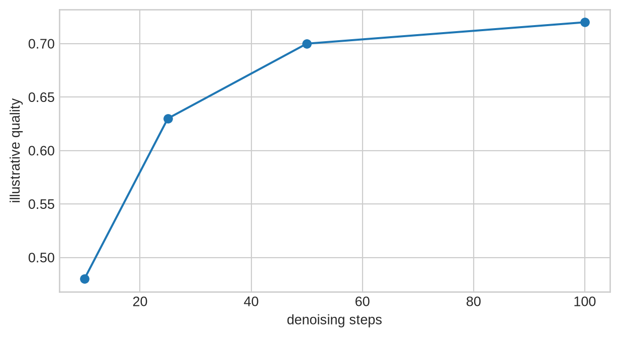
A denoising budget determines how long a user waits, how many accelerators are required, and how many outputs can be produced under a cost limit. It also determines the distribution of failure: a low step count may preserve broad category while losing fine relations; a high step count may improve some conditions and merely consume more time on others. Measure marginal gains by task slice and establish a stopping or fallback rule. For example, an interactive preview may use a low budget, while a final export receives more steps after a user confirms the condition.
The policy should make this distinction visible. A preview is not evidence that the final output will satisfy a condition; a final output should identify its generation settings where reproducibility matters. Cancellation, timeout, and retry rules need the same care as the sampler itself. A repeated request with a new seed may be a legitimate diversity control, while an automatic retry after a failed edit can overwrite a user decision if it is not bounded.
## Level 4 - Evaluation, deployment, and limits
### Evaluation protocols should resist selective sampling
Generated images are easy to curate after the fact. A credible protocol fixes prompts or source images, seeds or seed-selection policy, output count, sampler settings, and evaluation criteria before generation. If human reviewers compare outputs, randomise presentation order and hide model identity where feasible. Report reviewer instructions, disagreement, exclusions, and whether reviewers saw the original condition. Automated measures should be accompanied by the feature extractor, preprocessing, sample count, and confidence interval.
Failure categories should be defined before inspection but refined transparently if new failures appear. Useful categories include condition omission, relation error, object-count error, unreadable text, identity drift, unwanted edit outside a mask, unsafe content, and corrupted output. Count categories by condition slice rather than selecting memorable failures. A system that performs well on common prompts but fails on low-light inputs, unusual languages, or small objects has a bounded capability that should be stated directly.
### Reproducibility and change control
Diffusion results depend on many coupled software components. Updating a text encoder, latent decoder, scheduler library, precision kernel, safety filter, or prompt template can change output without a new denoiser checkpoint. Preserve versions and hashes where the environment permits, and retain a small fixed regression suite of conditions, seeds, and source images. Run it whenever a component changes. Visual inspection is useful, but a change log and predefined checks provide stronger evidence that a new release has not silently altered expected behaviour.
The regression suite should include both desired and undesired requests. It can test that a permitted edit preserves an unmasked region, that a condition is followed within a stated tolerance, that an unsupported request is handled according to policy, and that latency remains within a budget. This is the link between a generative model chapter and the operational material in Chapter 48: the deployed system includes model, sampler, interface, controls, and monitoring.
### Research claims need an appropriate comparison
Diffusion papers and systems often compare architecture, schedule, sampler, guidance, latent representation, or conditioning method at the same time. A reader should ask what is actually held fixed. If one model is trained at higher resolution, uses a different encoder, has more sampling steps, or receives a more favourable prompt protocol, a difference in displayed samples cannot be assigned to one architectural component. Ablations are useful when they preserve the relevant data, training budget, evaluation set, and output protocol.
Comparisons with autoregressive or adversarial generators require the same discipline. Diffusion offers an iterative denoising route; it does not make quality, diversity, controllability, or cost automatically superior for every task. State the resolution, quality and adherence criterion, hardware, latency percentile, sample count, and condition distribution. A system decision can then weigh the observed trade-off rather than rely on a category label.
### Questions that remain open in a deployment
Several limits are empirical. It is difficult to know whether an apparent visual relation was learned from a condition or produced through a frequent association. It is difficult to measure memorisation over a large and partly undocumented training corpus. It is difficult to compare quality across prompts that have many valid outputs, and to distinguish an unsafe request from an allowed creative transformation without a task-specific policy. These uncertainties should lead to narrower claims and continued monitoring, not to a generic disclaimer.
For a deployed generator, the accountable organisation must decide which evidence is sufficient for a particular use, which failures require human review, what data and outputs are retained, and how users can contest or report a result. The denoising mechanism explains how samples are produced. It does not decide whether a sample is appropriate, lawful, or reliable in a given workflow.
The practical lesson is to keep generation decisions inspectable. A request should be traceable to a condition, model version, sampler, budget, output policy, and evaluation boundary. An evaluation should identify the task property it measures and the populations or requests it leaves uncertain. With those records, a diffusion model can be compared, revised, or withdrawn on evidence. Without them, impressive samples can conceal an unmeasured system.
Those records also make later replication possible when hardware, libraries, interfaces, and policies inevitably change after the original experiment or release.
They support audit, comparison, and accountable correction.
```{python}
#| label: fig-reverse-chain
#| fig-cap: "Sampling applies the learned denoiser repeatedly, moving from noise through intermediate states to an image sample."
#| fig-alt: "A row of boxes flows from noise through three denoising steps to a generated image."
from matplotlib.patches import Rectangle, FancyArrowPatch
fig,ax=plt.subplots(figsize=(8,2.5));ax.axis("off")
for i,label in enumerate(["noise","step T","step T/2","step 1","sample"]):
 ax.add_patch(Rectangle((.2+i*1.55,1),1.1,.48,facecolor=["#7655a6","#d97745","#3a9188","#24527a","#3a9188"][i],edgecolor="white"));ax.text(.75+i*1.55,1.24,label,ha="center",va="center",color="white",fontsize=9)
ax.set_xlim(0,8);ax.set_ylim(.5,2);plt.show()
```
### Conditional-generation record
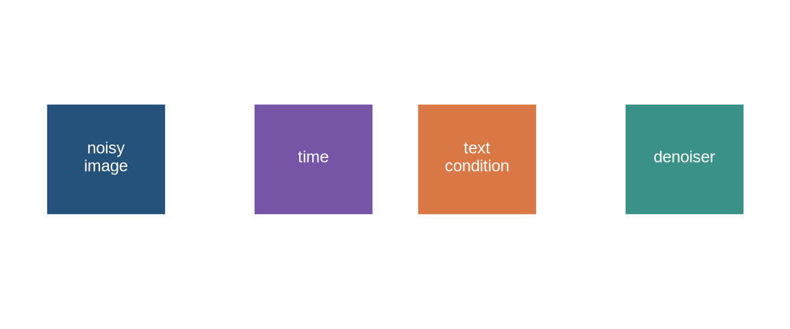
Conditioning supplies information that the reverse model should respect: a class label, text representation, masked image region, or another image. The condition is an input to the denoiser, not proof that every sample follows it. Evaluate adherence separately from visual quality, and retain the text encoder, guidance scale, negative condition, scheduler, seed policy, and resolution in the generation record.
```{python}
#| label: fig-conditioning
#| fig-cap: "A conditional diffusion model combines a noisy image, time representation, and condition before predicting a denoising direction."
#| fig-alt: "Noisy image, time step, and text condition arrows enter a denoiser and produce a noise prediction."
fig,ax=plt.subplots(figsize=(7.5,3));ax.axis("off")
for x,l,c in [(.3,"noisy\nimage","#24527a"),(2.2,"time","#7655a6"),(3.7,"text\ncondition","#d97745"),(5.6,"denoiser","#3a9188")]:ax.add_patch(Rectangle((x,1),1.1,.55,facecolor=c,edgecolor="white"));ax.text(x+.55,1.28,l,ha="center",va="center",color="white",fontsize=9)
ax.set_xlim(0,7);ax.set_ylim(.5,2);plt.show()
```
### Output evaluation and data-provenance boundary
Image-quality scores compare generated and reference distributions under a specific feature extractor and sample protocol. They do not establish prompt adherence, representation of rare groups, absence of memorisation, or suitability for a particular user task. Report data provenance, filtering, resolution, conditioning, sampler, steps, guidance, seeds, compute, and failure slices.
Evaluation should retain individual samples and prompts alongside aggregate scores. Inspect failures by requested relation, object count, text rendering, low-frequency visual structure, sensitive attribute, and training-data proximity. For applications with a user-facing claim, the relevant question is whether the stated condition is respected under that workflow, not whether samples look plausible after selective inspection.
Memorisation and provenance require a separate audit. Nearest-neighbour checks against training and evaluation data can detect some suspiciously close outputs, but they cannot demonstrate the absence of training-data reproduction. Record data collection and filtering, opt-out and removal procedures, known copyrighted or sensitive material, and the conditions under which a sample may be retained for review. These are deployment decisions with consequences beyond a feature-based image-quality score.
```{python}
#| label: fig-step-quality-cost
#| fig-cap: "More denoising steps can improve a stated quality measure while increasing generation latency; the curve must be measured for the chosen sampler and condition."
#| fig-alt: "A curve rises and flattens as denoising steps increase, while a second axis represents increasing latency."
steps=np.array([10,25,50,100]);quality=np.array([.48,.63,.70,.72]);fig,ax=plt.subplots(figsize=(6.5,3.6));ax.plot(steps,quality,marker="o");ax.set_xlabel("denoising steps");ax.set_ylabel("illustrative quality");plt.tight_layout();plt.show()
```
## Common misconceptions
- **Diffusion creates an image in one denoising call.** Sampling is normally iterative.
- **A lower noise-prediction loss proves better conditional images.** Adherence and visual quality require separate evaluation.
- **More steps always justify their cost.** The quality-latency curve depends on sampler and task.
- **A conditional prompt guarantees content.** Conditions steer a distribution and can be ignored or only partly followed.
## Exercises
1. Describe forward corruption and reverse denoising.
2. Explain why time is an input to the denoiser.
3. Plot a schedule with decreasing signal share.
4. Compare 25 and 100 denoising steps under a latency budget.
5. Define a conditional-adherence metric.
6. State a generation-record field required for reproducibility.
7. Explain why seed policy matters.
8. Design a failure slice for small objects.
9. Distinguish training noise from sampling noise.
10. Explain what a feature-based quality score does not measure.
11. Compare two schedules with equal end noise.
12. Identify a data-provenance risk.
13. Propose an intervention for condition adherence.
14. State how resolution changes cost.
15. Describe a sampler comparison protocol.
16. Identify the next chapter's multimodal question.
## Summary
Diffusion models learn denoising across a declared noise schedule and generate through repeated reverse steps. The sampler, condition, and evaluation protocol define the system's practical behaviour.
## Looking ahead
Diffusion provides one route from a learned representation to generated images, but applications often require a model to coordinate more than one modality. [Chapter 46](46-multimodal-models.qmd) examines the interfaces and objectives needed to align text, images, and other inputs without treating cross-modal performance as a single undifferentiated capability.
## Further reading
DDPM is introduced by @ho2020ddpm. Faster implicit sampling is developed by @song2020ddim.