---
title: "Full and Parameter-efficient Fine-tuning"
subtitle: "Changing a model for a task while controlling memory, storage, and regressions"
---
## The problem
The adaptation objectives in Chapters 29 and 30 both update a checkpoint, but neither said which parameters the update may touch. Full fine-tuning updates all trainable model parameters. That freedom has a price: gradients and optimiser state for every weight must fit in memory, every run produces a complete new checkpoint, and serving several task variants means storing several full models.
Parameter-efficient fine-tuning (PEFT) trades some of that freedom for control over cost. It freezes most base weights and trains a smaller set of added or selected parameters, so task-specific changes can be stored separately and different adaptations can load over one base model. The choice affects optimiser memory, checkpoint storage, deployment, multi-task serving, and the kinds of changes a run can represent. Neither method removes the need for data documentation or evaluation: a small adapter can overfit, encode an unsafe behaviour, or fail outside its tuning distribution, and a full update can improve a target task while degrading retained behaviours. This chapter gives the comparison and the implementation contracts required to make it interpretable.
### One linear layer makes the update visible
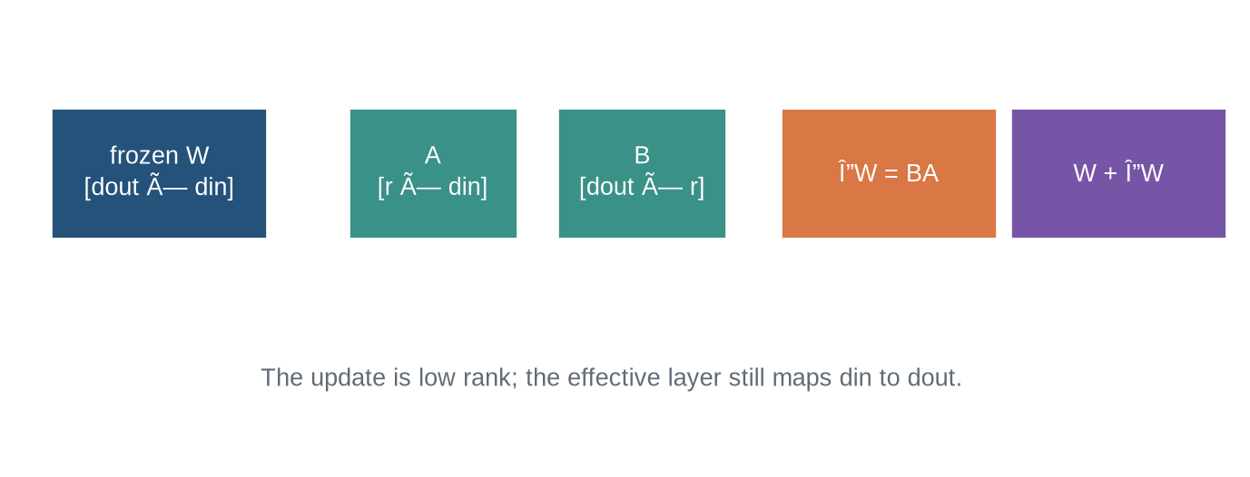
The running example is a linear layer with base weight $W$. LoRA learns a low-rank update $\Delta W = BA$ instead of a full-size change to $W$. The base weight remains frozen during training, and the update can be applied separately at inference or merged into a copy of the base weight.
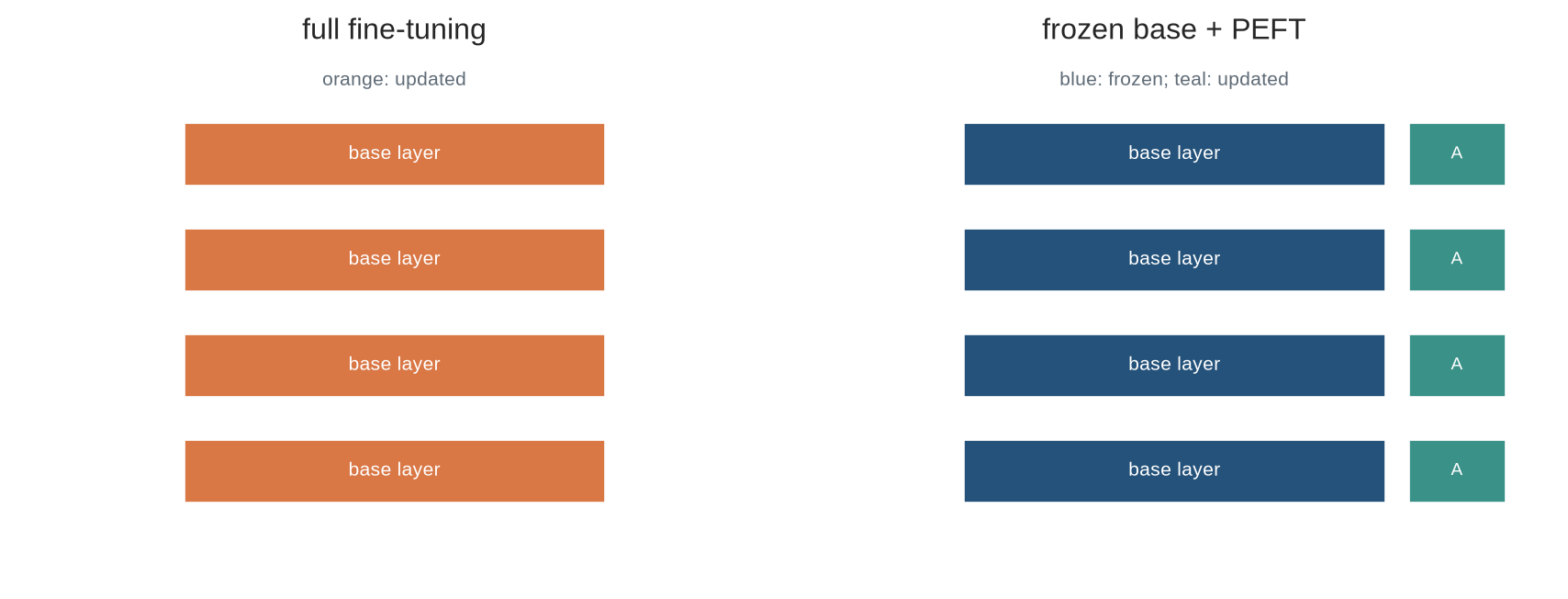
The first diagram contrasts the two methods on the same stack of layers. In the left panel every base layer is orange: all of them update. In the right panel the base layers stay blue and frozen, and only the small teal modules attached to them are trainable. Notice what the right panel hides: the frozen weights still participate in every forward computation, so freezing changes what is learned, not what is used.
```{python}
#| label: fig-full-vs-peft
#| fig-cap: "Full fine-tuning updates every base parameter, while parameter-efficient adaptation freezes the base and trains a smaller update module."
#| fig-alt: "Two diagrams contrast all layers marked trainable with base layers frozen and small adapter modules marked trainable."
import numpy as np
import matplotlib.pyplot as plt
from matplotlib.patches import Rectangle
plt.style.use("seaborn-v0_8-whitegrid")
blue,teal,orange,purple,grey="#24527a","#3a9188","#d97745","#7655a6","#5f6b76"
fig,axes=plt.subplots(1,2,figsize=(9,3.5))
for ax,title,mode in zip(axes,["full fine-tuning","frozen base + PEFT"],["full","peft"]):
    ax.axis("off"); ax.set_title(title)
    for i in range(4):
        y=.15+i*.2; c=orange if mode=="full" else blue
        ax.add_patch(Rectangle((.22,y),.56,.12,facecolor=c,edgecolor="white")); ax.text(.5,y+.06,"base layer",ha="center",va="center",color="white",fontsize=8)
        if mode=="peft": ax.add_patch(Rectangle((.81,y),.13,.12,facecolor=teal,edgecolor="white")); ax.text(.875,y+.06,"A",ha="center",va="center",color="white",fontsize=7)
    ax.text(.5,.94,"orange: updated" if mode=="full" else "blue: frozen; teal: updated",ha="center",color=grey,transform=ax.transAxes,fontsize=8)
plt.tight_layout(); plt.show()
```
That distinction governs the chapter. The trainable fraction can be a thousandth of the base, yet the base must still be stored, loaded, and executed, and the adapter means nothing apart from the exact base it was trained against.
::: {.concept-box .concept-core #concept-fine-tuning data-term="Fine-tuning and PEFT" data-domain="Large language models"}
**Fine-tuning and parameter-efficient fine-tuning.** Fine-tuning updates a pretrained checkpoint for a declared task. Full fine-tuning updates selected base parameters; PEFT retains most base weights and trains a smaller update module.
:::
::: {.concept-box .concept-distinction #concept-full-peft data-term="Full and parameter-efficient fine-tuning" data-domain="Large language models"}
**Full and parameter-efficient fine-tuning.** Full fine-tuning changes broad base-model state. Parameter-efficient methods constrain trainable updates to selected modules or low-rank changes. The comparison includes task outcomes, memory, storage, and serving compatibility.
:::
## Level 1 - Intuition
### Adaptation changes a checkpoint under a task distribution
Full fine-tuning applies gradients to all selected model weights. It can represent broad changes, but it requires storing gradients and optimiser state for those weights and usually produces a full new checkpoint. Parameter-efficient methods retain the base checkpoint and train a smaller module, such as low-rank matrices, adapters, prompts, or selected bias terms. This makes it possible to store task-specific changes separately and load different adaptations over one base model.
The methods are not ordered by quality in the abstract. The relevant comparison depends on task complexity, data size, available hardware, update frequency, latency constraints, compatibility requirements, and the cost of keeping several adapted versions. A smaller update reduces trainable parameters; it does not make the task specification or evaluation smaller.
```{python}
base_parameters=7_000_000_000
adapter_parameters=8_000_000
print("trainable fraction:",adapter_parameters/base_parameters)
```
### Frozen weights are still part of the function
A PEFT adapter is not a standalone model. It assumes a particular base checkpoint, architecture, tokenizer, layer naming convention, target modules, rank, scaling rule, and often quantisation configuration. Loading an adapter onto a related model with the same visible size can change or break its function. The serving record must bind the adapter to its compatible base.
```{python}
adapter_metadata={"base":"checkpoint-v1","target_modules":["q_proj","v_proj"],"rank":8,"scale":16}
print(adapter_metadata)
```
Level 1 framed adaptation as a choice of what to update and what to freeze. Level 2 makes the low-rank update concrete: its parameter count, its scaling, and the merge operation that prepares it for inference.
## Level 2 - Mechanics
### Low-rank updates reduce trainable parameter count
For a layer $W\in\mathbb{R}^{d_{out}\times d_{in}}$, a full update contains $d_{out}d_{in}$ parameters. A rank-$r$ LoRA update uses $A\in\mathbb{R}^{r\times d_{in}}$ and $B\in\mathbb{R}^{d_{out}\times r}$, for $r(d_{in}+d_{out})$ trainable parameters. The update is commonly scaled by a factor such as $\alpha/r$ [@hu2021lora].
```{python}
d_in,d_out,r=4096,4096,8
full=d_in*d_out; lora=r*(d_in+d_out)
print("full parameters:",full,"LoRA parameters:",lora,"fraction:",lora/full)
```
```{python}
#| label: fig-low-rank-update
#| fig-cap: "A low-rank adapter represents a large weight update through two smaller matrices whose product has the base layer's shape."
#| fig-alt: "A diagram shows an input dimension through a rank-eight bottleneck to an output dimension, with the product added to a frozen base matrix."
fig,ax=plt.subplots(figsize=(9,3.3)); ax.axis("off")
for x,w,label,c in [(.25,1.6,"frozen W\n[dout × din]",blue),(2.45,1.25,"A\n[r × din]",teal),(4.0,1.25,"B\n[dout × r]",teal),(5.65,1.6,"ΔW = BA",orange),(7.35,1.6,"W + ΔW",purple)]:
    ax.add_patch(Rectangle((x,1.25),w,.62,facecolor=c,edgecolor="white")); ax.text(x+w/2,1.56,label,ha="center",va="center",color="white")
ax.text(4.4,.55,"The update is low rank; the effective layer still maps din to dout.",ha="center",color=grey); ax.set_xlim(0,9); ax.set_ylim(.2,2.3); plt.show()
```
The reduction is largest when rank is much smaller than layer widths. Targeting only some projections reduces it further. These decisions restrict the trainable update family. They can be sufficient for a task, but sufficiency should be demonstrated on target and retained evaluations, not inferred from a low training loss.
### Merge and unmerge are numerical operations
At inference, an adapter can be applied as a separate branch or merged by forming $W' = W + sBA$. Merging can reduce runtime overhead, but it creates a new effective weight tensor. Repeated merging, wrong scaling, mismatched dtype, or merging into the wrong base can produce irreversible errors unless the original base and adapter are retained.
```{python}
np.random.seed(2)
W=np.random.randn(3,4); A=np.random.randn(2,4); B=np.random.randn(3,2); scale=.5
x=np.random.randn(4)
separate=W@x+scale*(B@(A@x))
merged=(W+scale*B@A)@x
assert np.allclose(separate,merged)
print("separate and merged adapter outputs agree")
```
Level 2 derived the update and verified merge equivalence in arithmetic. Level 3 counts the resources: what training memory actually consists of when the base is frozen, and how module scope changes the trainable family.
## Level 3 - Mathematics & Code
### Trainable parameters are not the whole memory account
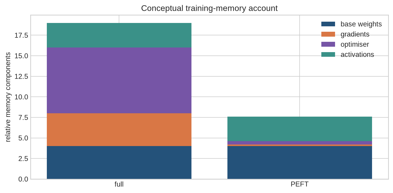
Training memory includes base weights, trainable weights, gradients, optimiser states, activations, temporary buffers, and communication state. Freezing a base model can remove its gradient and optimiser-state requirements, but the base weights and many forward activations remain. Quantising frozen weights can lower storage further, while introducing a new numerical configuration that must be evaluated. QLoRA combines quantised base weights with low-rank adapters [@dettmers2023qlora].
```{python}
params=7_000_000_000; bytes_per_weight=2; bytes_per_adam_state=8
full_weight_gib=params*bytes_per_weight/2**30
full_adam_gib=params*bytes_per_adam_state/2**30
print("base weights GiB:",round(full_weight_gib,1),"Adam moments GiB:",round(full_adam_gib,1))
```
```{python}
#| label: fig-memory-account
#| fig-cap: "Freezing base weights changes gradient and optimiser-state requirements, but base-weight and activation memory remain in the training account."
#| fig-alt: "Stacked conceptual bars compare full fine-tuning and PEFT memory components: base weights, gradients, optimiser state, and activations."
fig,ax=plt.subplots(figsize=(8,4)); categories=["base weights","gradients","optimiser","activations"]; full=np.array([4,4,8,3]); peft=np.array([4,.2,.4,3]); bottom=np.zeros(2)
for vals,name,c in zip([np.array([full[i],peft[i]]) for i in range(4)],categories,[blue,orange,purple,teal]): ax.bar(["full","PEFT"],vals,bottom=bottom,label=name,color=c); bottom+=vals
ax.set_ylabel("relative memory components"); ax.legend(); ax.set_title("Conceptual training-memory account"); plt.tight_layout(); plt.show()
```
### Parameter scope is a substantive design choice
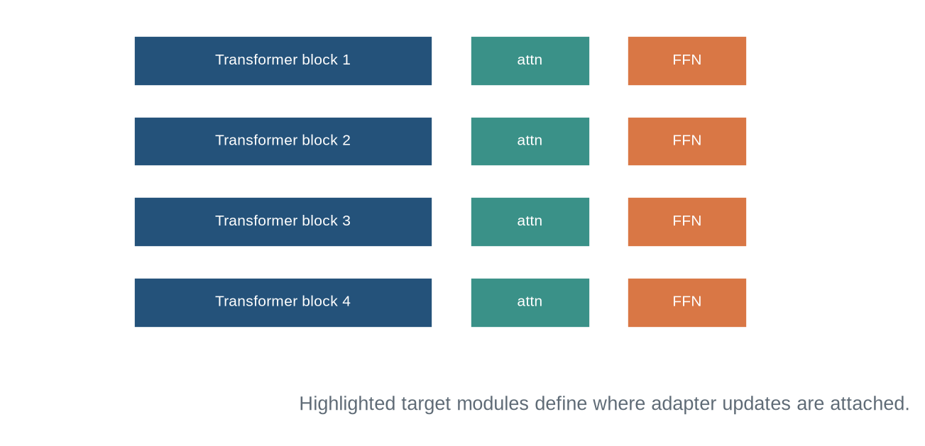
PEFT is a family of methods rather than one fixed architecture. An implementation may target attention projections, feed-forward layers, output heads, selected biases, or inserted adapter blocks. Each scope changes which transformations can adapt and how many new parameters are trained. The scope should be reported at the level of module names and layer coverage, not only as a total trainable-parameter count.
Targeting all layers can permit a more distributed adaptation than targeting only a final projection. Targeting a small subset can reduce storage and training time while concentrating the burden of adaptation in fewer locations. The appropriate choice is empirical: test candidate scopes on the declared task and retained suite under the same data and optimisation budget.
```{python}
#| label: fig-module-scope
#| fig-cap: "Adapter placement can target selected attention and feed-forward projections or every compatible layer; the placement changes the trainable update family."
#| fig-alt: "A stack of Transformer blocks has highlighted adapter locations in attention projections and feed-forward layers."
fig,ax=plt.subplots(figsize=(8.5,4)); ax.axis("off")
for i in range(4):
    y=3.15-i*.72; ax.add_patch(Rectangle((.8,y),2.0,.45,facecolor=blue,edgecolor="white")); ax.text(1.8,y+.225,f"Transformer block {i+1}",ha="center",va="center",color="white",fontsize=8)
    ax.add_patch(Rectangle((3.05,y),.8,.45,facecolor=teal,edgecolor="white")); ax.text(3.45,y+.225,"attn",ha="center",va="center",color="white",fontsize=8)
    ax.add_patch(Rectangle((4.1,y),.8,.45,facecolor=orange,edgecolor="white")); ax.text(4.5,y+.225,"FFN",ha="center",va="center",color="white",fontsize=8)
ax.text(3.95,.25,"Highlighted target modules define where adapter updates are attached.",ha="center",color=grey); ax.set_xlim(0,6); ax.set_ylim(.05,3.8); plt.show()
```
Level 3 counted the training memory and the trainable update family. Level 4 turns to the operational decisions: adapter routing, checkpoint recoverability, the interaction of data volume and update scope, and the evidence a method selection requires.
## Level 4 - Research & Systems
### Multi-adapter serving creates routing decisions
Separate adapters can make several task variants cheaper to store than several full checkpoints. Serving still needs a policy for selecting the adapter, ensuring it is compatible with the request, batching requests that use different adapters, and preventing an adapter intended for one task or policy from being silently applied to another. An adapter identifier is part of the request and audit trace.
```{python}
routes={"legal-summary":"adapter-legal-v2","code-review":"adapter-code-v1"}
request_task="code-review"
print("selected adapter:",routes[request_task])
```
### Checkpoint organisation determines recoverability
An adaptation run should preserve the immutable base identifier, adapter weights, configuration, tokenizer and template versions, training state where resumption is required, and evaluation records. A merged weight file alone can make a task variant convenient to serve, but it loses the clean separation between base and update unless both original artefacts are retained. A safe workflow treats merging as a reproducible build step with an output hash and an equivalence test.
```{python}
checkpoint={"base_hash":"abc","adapter_hash":"def","merge_scale":16/8,"merged":False,"template":"v3"}
assert checkpoint["base_hash"] and checkpoint["adapter_hash"]
print("recoverable adapter checkpoint metadata present")
```
### Data volume and update scope interact
An adapter with few trainable parameters does not imply that many examples are required, nor does a full update imply that a small dataset is necessarily unsuitable. The relevant risk depends on how far the target distribution differs from the base model, how repetitive the data are, how many update tokens and epochs are used, and which evaluation tasks must remain stable. A small, tightly specified adaptation can overfit through either method when the validation split duplicates templates or sources.
Checkpoint selection should inspect learning curves and held-out behaviour across more than one update count. A model that reaches its best target score early may degrade after additional passes over narrow data. Retaining base and intermediate checkpoints makes it possible to compare the adaptation trajectory rather than selecting only the final artifact.
```{python}
history={"step_100":{"target":.58,"retained":.71},"step_500":{"target":.66,"retained":.69},"step_900":{"target":.65,"retained":.62}}
for step,metrics in history.items(): print(step,metrics)
```
### Choose an adaptation method against a declared constraint
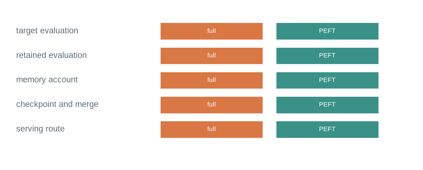
An adaptation plan should specify the base checkpoint, task, data provenance, target modules or full parameter scope, rank and scaling where relevant, quantisation and precision, maximum length, optimiser settings, token budget, checkpoint policy, merge status, and serving route. It should report target-task results and a retained-task suite under the same prompt template and decoding policy.
```{python}
#| label: fig-selection-audit
#| fig-cap: "Adaptation selection compares full and parameter-efficient methods against target quality, regressions, training resources, storage, and serving constraints."
#| fig-alt: "A table-like diagram compares full fine-tuning and PEFT across target evaluation, regression suite, memory account, checkpoint size, and serving route."
fig,ax=plt.subplots(figsize=(9,3.5)); ax.axis("off")
rows=["target evaluation","retained evaluation","memory account","checkpoint and merge","serving route"]
for i,row in enumerate(rows):
    y=2.7-i*.48; ax.text(.2,y,row,va="center",color=grey); ax.add_patch(Rectangle((3.0,y-.17),2,.34,facecolor=orange,edgecolor="white")); ax.text(4,y,"full",ha="center",va="center",color="white",fontsize=8); ax.add_patch(Rectangle((5.25,y-.17),2,.34,facecolor=teal,edgecolor="white")); ax.text(6.25,y,"PEFT",ha="center",va="center",color="white",fontsize=8)
ax.set_xlim(0,8); ax.set_ylim(.1,3.2); plt.show()
```
The method should not be selected solely because it is cheaper or because it reaches the lowest training loss. A full update may be necessary for a target distribution; a low-rank update may be sufficient and operationally preferable. Both conclusions require evidence under the specified task and deployment conditions.
### Regression tests should include the base interface
Adaptation can change outputs for prompts outside the fine-tuning corpus. Retained tests should include general instruction responses, domain tasks that must remain available, formatting or tool contracts, and safety-sensitive inputs where relevant. Tests must specify whether the adapter is active and which system template is used. Comparing a base checkpoint without its standard template to an adapter checkpoint with a richer interface would not isolate the update.
```{python}
results={"target":{"base":.48,"adapter":.67},"retained":{"base":.72,"adapter":.70}}
for suite,scores in results.items(): print(suite,scores)
```
## Common misconceptions
- **PEFT changes only a few values, so it cannot cause a large behavioural change.** Small modules can substantially change the effective function.
- **An adapter can be used with any model of the same size.** It requires the compatible base and architecture contract.
- **Freezing the base eliminates training memory demands.** Base weights and activations remain.
- **Merged and separate adapters always give the same result without qualification.** Scaling, dtype, and correct base identity are required.
- **A lower training loss identifies the best adaptation method.** Target, retained, and systems constraints require separate evidence.
## Exercises
1. Calculate LoRA parameters for stated layer widths and rank.
2. Compare full-update and low-rank-update parameter counts.
3. Verify merged and separate LoRA outputs on a toy layer.
4. List adapter metadata needed for safe loading.
5. Explain which training memory components remain when a base is frozen.
6. State how quantisation changes an adaptation record.
7. Design a multi-adapter routing trace.
8. Compare adapter storage with a full checkpoint for several tasks.
9. Identify a merge error and a test that detects it.
10. Specify target and retained evaluation suites for an adaptation.
11. Explain why rank is a model-selection parameter.
12. Describe an evaluation for a template mismatch.
13. State why a PEFT update can still overfit.
14. Compare training and serving implications of merged adapters.
15. List fields required in an adaptation run record.
16. Identify the chapter that treats quantisation and efficient inference.
## Summary
Full fine-tuning updates selected base parameters, while parameter-efficient methods train smaller updates over a frozen checkpoint. LoRA represents one such update as a low-rank matrix product. The choice changes trainable parameter count, optimiser state, checkpoint storage, and serving design, but it does not remove the need for task data, compatibility metadata, or regression evaluation.
[Chapter 32](32-quantisation-efficient-inference.qmd) examines lower-precision weights and activations as a separate efficiency and accuracy trade-off.
## Looking ahead
Adaptation changes the model or an attached update. [Chapter 32](32-quantisation-efficient-inference.qmd) examines how the resulting tensors can be represented and executed under tighter memory and latency constraints.
## Further reading
LoRA is introduced by @hu2021lora. QLoRA studies low-rank adaptation with quantised base models [@dettmers2023qlora].