Vision Transformers

Image patches, positional structure, attention, and visual evaluation

Chapter orientation

Why this chapter matters

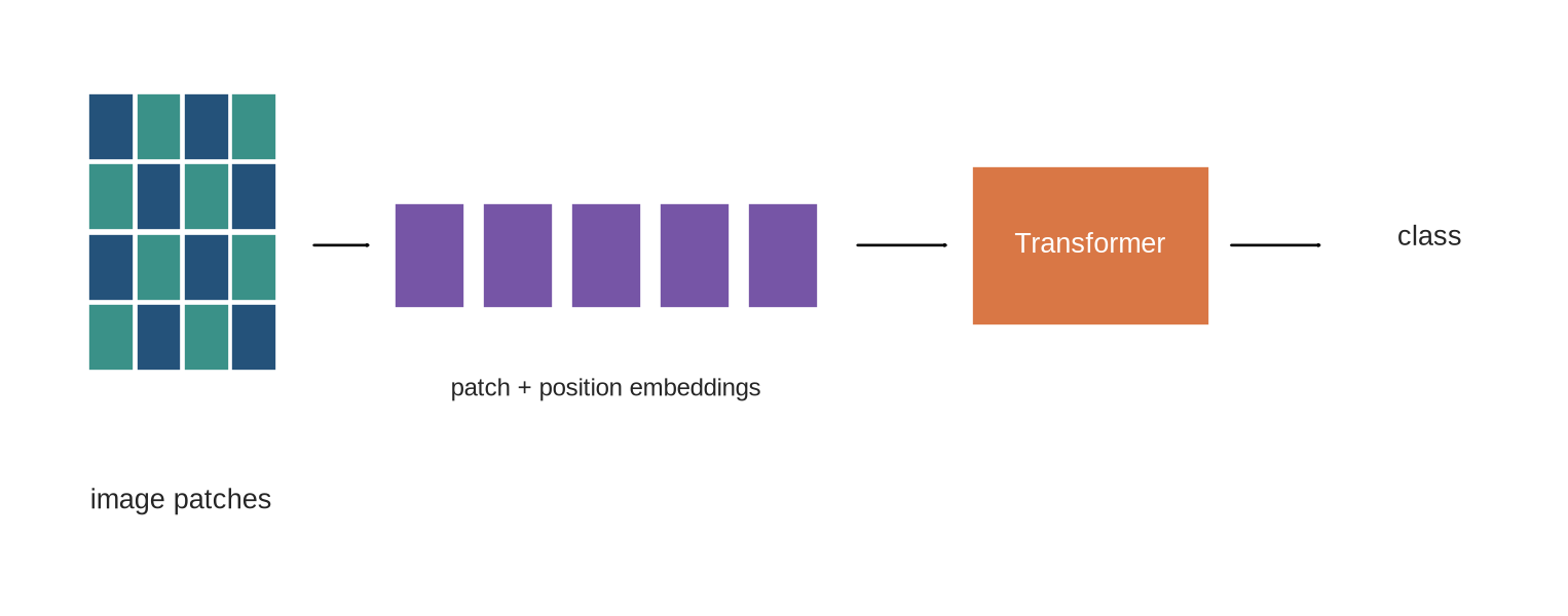
Transformers expect a sequence of vector representations. A vision transformer (ViT) constructs that sequence by dividing an image into fixed-size patches, mapping each patch to an embedding, adding positional information, and applying Transformer blocks. The architecture therefore reuses the representation, attention, and positional mechanisms developed in Chapters 16-23, while changing the meaning and number of tokens.

An image is not a sequence of words. Patch size determines what visual detail enters the model, positional embeddings supply spatial order, and attention provides global token interactions. The original ViT showed that a pure Transformer over patch sequences can perform strongly when pretrained at sufficient scale (Dosovitskiy et al. 2021). Training regime matters: data-efficient ViTs use augmentation and distillation choices that change the comparison with convolutional models (Touvron et al. 2021).

Learning objectives

By the end of this chapter, you should be able to:

• calculate the number of image patches and resulting attention-token cost;
• explain patch projection, positional embeddings, and a classification representation;
• distinguish spatial information supplied by patches from information supplied by position;
• compare global attention with convolutional locality under declared conditions; and
• design an image-classification evaluation that reports resolution, preprocessing, and data shifts.

Vision Transformer. A Transformer-based visual model that converts an image into patch representations and processes them as a sequence. Patch size, preprocessing, resolution, and positional information are part of the visual interface.

Level 1 - Images become token sequences

Patchification determines the visual interface

For an image of height (H) and width (W), square patches of side (P) produce (N=(H/P)(W/P)) tokens when the dimensions divide exactly. Each flattened patch is projected into the model dimension. The projection does not preserve every pixel relationship explicitly; it supplies a learned representation from which later layers must recover useful visual structure.

import numpy as np
import matplotlib.pyplot as plt
from matplotlib.patches import Rectangle, FancyArrowPatch
plt.style.use("seaborn-v0_8-whitegrid")
blue,teal,orange,purple,grey="#24527a","#3a9188","#d97745","#7655a6","#5f6b76"
fig,ax=plt.subplots(figsize=(10,3.8)); ax.axis("off")
for i in range(4):
 for j in range(4): ax.add_patch(Rectangle((.4+i*.28,1.3+j*.28),.27,.27,facecolor=blue if (i+j)%2 else teal,edgecolor="white"))
ax.text(.95,.75,"image patches",ha="center")
for i in range(5): ax.add_patch(Rectangle((2.2+i*.52,1.55),.42,.42,facecolor=purple,edgecolor="white"))
ax.add_patch(FancyArrowPatch((1.7,1.8),(2.1,1.8),arrowstyle="-|>")); ax.text(3.45,1.2,"patch + position embeddings",ha="center",fontsize=9)
ax.add_patch(FancyArrowPatch((4.9,1.8),(5.5,1.8),arrowstyle="-|>")); ax.add_patch(Rectangle((5.6,1.48),1.4,.64,facecolor=orange,edgecolor="white")); ax.text(6.3,1.8,"Transformer",ha="center",va="center",color="white")
ax.add_patch(FancyArrowPatch((7.1,1.8),(7.7,1.8),arrowstyle="-|>")); ax.text(8.3,1.8,"class",ha="center"); ax.set_xlim(0,9); ax.set_ylim(.4,2.7); plt.show()

Figure 45.1: A vision transformer divides an image into patches, projects them to embeddings, adds positional information, and processes the resulting token sequence.

H=W=224; P=16; N=(H//P)*(W//P)
print({"patches":N,"tokens_with_class":N+1})

{'patches': 196, 'tokens_with_class': 197}

Patch projection fixes channels, scale, and patch boundaries

Patchification begins with a specific image representation: colour channels, value range, orientation, resizing policy, and crop. Flattening a 16-by-16 RGB patch produces a vector with 768 scalar values before projection; a grayscale image or a multispectral image has a different input dimension and cannot use the same projection without an explicit adaptation. The patch projection is therefore an interface between image acquisition and the Transformer, not a generic conversion from pixels to tokens.

Patch boundaries also matter. An object or edge can fall across two patches, a crop can remove a small object, and resampling can blur the feature that a downstream label depends on. Smaller patches expose more local detail but do not guarantee that the model will use it; larger patches can be sufficient when the visual signal is coarse. Store the resize, crop, channel, and patch policy with the checkpoint and evaluate the same policy on the held-out images.

Resolution and patch size are model choices

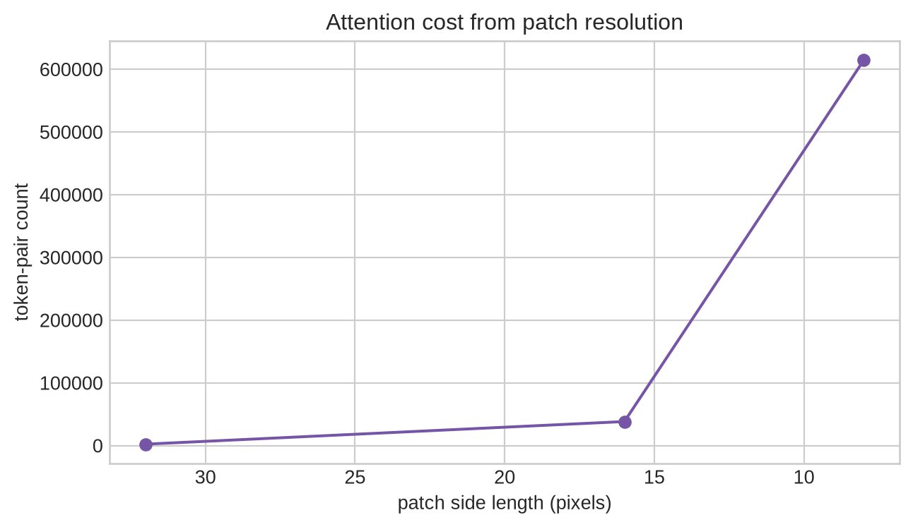
Smaller patches retain finer detail but create more tokens. Since full self-attention compares token pairs, the attention-score matrix grows approximately with (N^2). A 224-by-224 image with 16-by-16 patches gives 196 patch tokens; halving patch side length gives 784. The later model may have more visual detail available, but it also has a much larger attention computation and memory requirement.

sizes=np.array([32,16,8]); tokens=(224//sizes)**2
fig,ax=plt.subplots(figsize=(6.8,4)); ax.plot(sizes,tokens**2,marker="o",color=purple); ax.invert_xaxis(); ax.set_xlabel("patch side length (pixels)"); ax.set_ylabel("token-pair count"); ax.set_title("Attention cost from patch resolution"); plt.tight_layout(); plt.show()

Figure 45.2: Smaller image patches create more visual tokens and increase the quadratic attention relation count.

Resolution changes both evidence and computation

Increasing resolution can reveal a small object, text, or boundary that was absent from a lower-resolution input. It also changes the number of positions the model must process and the memory needed for attention. A comparison between two resolutions is therefore not a pure systems benchmark: it changes the information available to the classifier as well as the cost. Report the acquisition resolution, resize rule, crop selection, patch size, token count, and evaluation distribution together.

Position representations need a declared treatment when image grids change. A learned position table trained for one patch grid may be interpolated, resized, replaced, or used only at its original resolution. Each choice changes the input contract. Test performance at the intended resolution and, if resolution transfer is claimed, on a separately reported set rather than assuming that a position representation will generalise without loss.

Level 2 - Position and attention

Patches require an explicit spatial contract

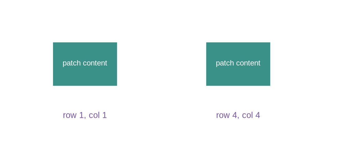
Flattening patches produces a sequence but does not itself specify where each patch came from. Learned or fixed positional embeddings add location information before the Transformer blocks. Without them, permuting patch order leaves the attention mechanism equivariant to that permutation, as in Chapter 21. Position tells the model that a patch came from the upper left rather than the lower right; it does not by itself supply translation invariance or local edge detectors.

fig,ax=plt.subplots(figsize=(7,3.3)); ax.axis("off")
for x,pos in [(1.0,"row 1, col 1"),(4.3,"row 4, col 4")]:
 ax.add_patch(Rectangle((x,1.5),1.4,.55,facecolor=teal,edgecolor="white")); ax.text(x+.7,1.78,"patch content",ha="center",va="center",color="white",fontsize=9); ax.text(x+.7,1.1,pos,ha="center",color=purple)
ax.set_xlim(0,7); ax.set_ylim(.6,2.5); plt.show()

Figure 45.3: Patch embeddings identify local visual content, while positional embeddings identify the patch’s place in the image grid.

Spatial position and visual invariance are different requirements

Position embeddings identify where a patch occurs in the processed image grid. They do not specify whether a class should remain unchanged after translation, crop, rotation, scale change, illumination shift, or a new camera. Some transformations should leave a label stable; others should not. A medical image label may depend on a small position change, while an object-class label may not. The appropriate invariance is a property of the task and data-generating process, not of the word Transformer.

Specify which transformations are represented in training augmentation, which are held out for evaluation, and which make an image no longer comparable. An augmented crop that removes the labelled object changes the target rather than testing invariance. This distinction prevents an apparent robustness result from mixing valid visual variation with a changed task definition.

Global attention and local inductive bias differ

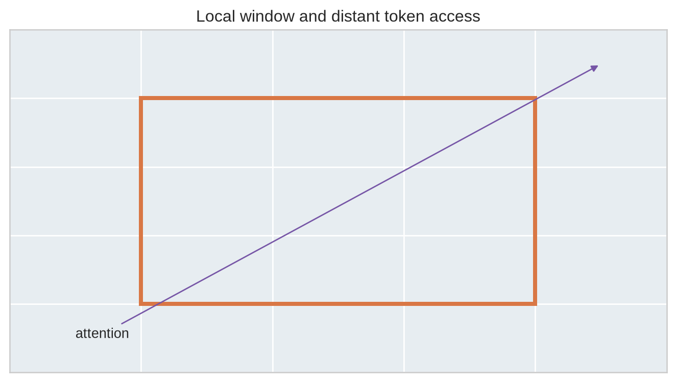
Convolution applies shared local filters and builds larger receptive fields across layers. ViT attention can connect distant patches directly within a layer. Neither property settles which model is preferable: the answer depends on data scale, augmentation, pretraining, resolution, compute, and the intended transfer task. A fair comparison fixes those conditions and reports them rather than treating architecture labels as results.

fig,ax=plt.subplots(figsize=(7,4)); ax.set_xticks([]); ax.set_yticks([])
for i in range(5):
 for j in range(5): ax.add_patch(Rectangle((i,j),1,1,facecolor="#e7edf1",edgecolor="white"))
ax.add_patch(Rectangle((1,1),3,3,fill=False,edgecolor=orange,lw=3)); ax.annotate("attention",xy=(4.5,4.5),xytext=(.5,.5),arrowprops={"arrowstyle":"-|>","color":purple}); ax.set_xlim(0,5); ax.set_ylim(0,5); ax.set_title("Local window and distant token access"); plt.tight_layout(); plt.show()

Figure 45.4: A convolutional layer begins with local neighbourhoods, whereas a ViT attention head can assign weight between distant patch tokens in one layer.

Architecture comparisons require matched visual evidence

Global attention and convolutional locality are architectural properties, but a reported image result also depends on the images and training policy available to each model. Match preprocessing, augmentation, label set, pretraining data boundary, optimiser, schedule, parameter or compute budget, resolution, and checkpoint-selection rule before attributing a difference to the architecture. The original ViT and data-efficient DeiT results illustrate how pretraining scale, augmentation, and distillation change the setting in which a visual Transformer is assessed (Dosovitskiy et al. 2021; Touvron et al. 2021).

The comparison should also define the prediction interface. A class token, average pooling, multi-scale feature aggregation, or a dense prediction head uses the final patch representations differently. A classification result does not establish object detection, segmentation, or localisation behaviour without a head, labels, and metrics for those tasks. Keep the claim at the task interface actually evaluated.

Level 3 - Training and representation checks

The classification representation is a declared interface

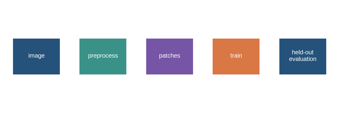
A classification ViT can prepend a learned class token and use its final representation for a classifier, or pool patch representations. These are different interfaces and should be reported. Training also inherits the earlier contracts: image normalisation, crop policy, augmentation, label mapping, optimiser, schedule, checkpoint selection, and the split used for final evaluation.

patches=np.array([[.2,.1],[.7,.3],[.1,.8]])
class_token=np.array([.5,.5]); sequence=np.vstack([class_token,patches])
print("sequence shape including class token:",sequence.shape)

sequence shape including class token: (4, 2)

Pretraining data and labels define the visual task

Pretraining can provide visual features that a small labelled dataset alone would not learn reliably. It can also introduce label definitions, geographic concentration, image-source conventions, or licensing and privacy constraints that differ from the deployment setting. Record the pretraining objective and data boundary separately from the fine-tuning dataset. A claim about transfer should identify which visual condition changed and which remained shared between pretraining and evaluation.

Label quality needs the same attention as architecture. A label may describe the whole image, a central object, a scene, a temporal state, or an annotator judgment. Crop and resize policies can change whether the labelled feature is visible. Inspect disagreement, class imbalance, missing labels, and the treatment of multi-label or ambiguous images before interpreting an apparent model error as a representation failure. The data and label contract determines the error that accuracy measures.

fig,ax=plt.subplots(figsize=(9,3)); ax.axis("off")
for i,(label,c) in enumerate([("image",blue),("preprocess",teal),("patches",purple),("train",orange),("held-out\nevaluation",blue)]):
 x=.2+i*1.75; ax.add_patch(Rectangle((x,1.25),1.25,.55,facecolor=c,edgecolor="white")); ax.text(x+.63,1.53,label,ha="center",va="center",color="white",fontsize=9)
ax.set_xlim(0,9); ax.set_ylim(.6,2.3); plt.show()

Figure 45.5: A ViT result depends on the image and training contract: preprocessing, patching, position, augmentation, labels, and evaluation split.

Training comparisons need checkpoint and augmentation controls

Augmentation may include random crops, flips, colour changes, masking, or mixing images and labels. These transformations can improve a model’s fit to a declared visual distribution, but they can also create examples that no longer support the original label. State the augmentation probability and order, the normalisation statistics, the optimisation schedule, and the criterion used to select the final checkpoint. Do not compare a ViT chosen from a large hyperparameter search with a baseline chosen from one run without recording the search policy.

Evaluate training stability as well as the selected checkpoint. Report variation across seeds or repeated runs where feasible, learning curves, and the relation between validation and held-out performance. A visual model can appear to improve because a crop policy matches one validation source unusually well. Preserving the split definition and checkpoint-selection record makes that possibility testable.

Level 4 - Evaluation and limits

Image accuracy is conditional on the visual distribution

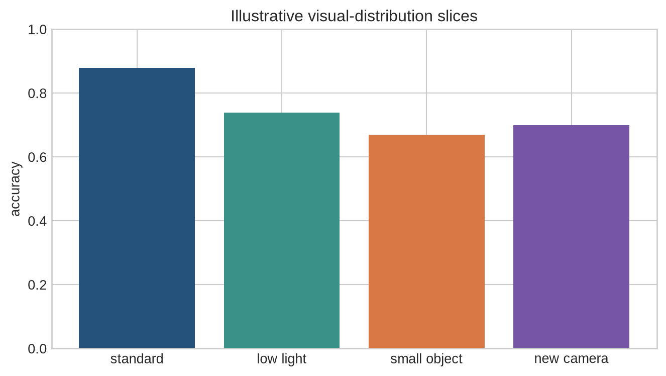
Image-classification results should report resolution, patch size, crop and normalisation policy, augmentation, pretraining data, class definitions, label quality, and test distribution. Evaluate slices where the visual task changes: viewpoint, lighting, background, object size, camera type, or geographic source. A high score on a fixed benchmark does not establish that the model recognises the same object under a changed acquisition process.

Attention maps can support an inspection of which patch relations received high weight. They do not on their own establish a causal explanation for the class prediction. Test an interpretation with interventions on patches, positional information, or the relevant visual feature, and report when the result is sensitive to preprocessing or patch boundaries.

Visual explanations need a prediction-changing intervention

An attention map, saliency map, or selected patch can be a useful hypothesis about which visual region matters. Test that hypothesis by masking, replacing, moving, or perturbing the specified region while preserving the task as far as possible, then measure the resulting prediction change. A patch that receives high attention but can be altered without affecting the result is not established as causally necessary. A prediction that changes after a broad blur or crop may reflect a preprocessing shift rather than the importance of one semantic object.

Record the intervention, the images selected for inspection, the baseline prediction, the transformed prediction, and any change in the model’s confidence or abstention decision. Visual explanations should be evaluated by image and slice; a convincing example can coexist with a procedure that fails on another acquisition condition. These records establish the limited claim that the intervention supports, not a general account of what the model sees.

Slice evaluation should distinguish acquisition, label, and representation failures

When performance falls on a visual slice, the source can be acquisition quality, a shifted class definition, label error, preprocessing mismatch, insufficient resolution, or a representation failure. Record the slice construction and inspect a bounded sample of errors before assigning cause. Low-light images may be darker because of a camera pipeline; small objects may be lost at the resize stage; a new geographic source may use another background or label convention. These are different interventions and need different responses.

For high-consequence image tasks, report abstentions, confidence calibration, review routes, and the consequences of false positives and false negatives by slice. A high aggregate accuracy cannot determine an appropriate decision threshold when the cost of errors differs across visual conditions. The evaluation record should make clear whether the model was assessed as a classifier, a triage aid, or a component that can defer to a human or another measurement process.

slices=["standard","low light","small object","new camera"]; acc=[.88,.74,.67,.70]
fig,ax=plt.subplots(figsize=(7,4)); ax.bar(slices,acc,color=[blue,teal,orange,purple]); ax.set_ylim(0,1); ax.set_ylabel("accuracy"); ax.set_title("Illustrative visual-distribution slices"); plt.tight_layout(); plt.show()

Figure 45.6: ViT evaluation should report performance by visual slice because changes in resolution, object scale, or acquisition conditions can alter the image distribution.

Common misconceptions

• Image patches are semantic objects. They are fixed spatial blocks projected into vectors.
• Position embeddings create visual invariance. They identify location; invariance must be learned or evaluated.
• Smaller patches are always better. They trade visual detail for token and attention cost.
• An attention map is a causal explanation. It is a weight pattern that needs an intervention test.
• ViT and convolutional models can be compared by architecture alone. Data, augmentation, resolution, pretraining, and compute affect the result.

Exercises

1. Calculate patch count for a 256-by-256 image with 16-by-16 patches.
2. Compare token-pair counts for 16 and 8 pixel patches.
3. Explain why position is needed after patch flattening.
4. State one spatial property that positional embeddings do not guarantee.
5. Implement a patch projection for a toy grayscale image.
6. Compare class-token and mean-pooling interfaces.
7. Draw a local convolutional receptive field and a distant attention relation.
8. Identify training-contract fields that affect a ViT comparison.
9. Design a low-light evaluation slice.
10. Explain how crop policy can change a label’s apparent difficulty.
11. Propose an intervention test for an attention-map interpretation.
12. State why a patch boundary can matter for a small object.
13. Compare dense attention cost at two image resolutions.
14. Specify a held-out visual distribution for transfer evaluation.
15. Identify a pretraining-data risk in image classification.
16. State the next chapter’s diffusion-model question.

Summary

Vision transformers turn images into patch-token sequences and use position-aware Transformer blocks to combine visual information. Patch size, position, training data, and evaluation distribution are part of the modelling contract. The architecture offers global token interactions, but its visual claims require evidence across the relevant image conditions.

Looking ahead

Patch-based Transformers describe how an image can be represented as a sequence; they do not specify how a new image is generated. Chapter 45 addresses that generative problem by treating image synthesis as a sequence of noise-removal decisions under a declared sampling procedure.

Further reading

Vision Transformer is introduced by Dosovitskiy et al. (2021). Data-efficient image Transformer training and distillation are studied by Touvron et al. (2021).

Dosovitskiy, Alexey, Lucas Beyer, Alexander Kolesnikov, et al. 2021. “An Image Is Worth 16x16 Words: Transformers for Image Recognition at Scale.” International Conference on Learning Representations. https://arxiv.org/abs/2010.11929.

Touvron, Hugo, Matthieu Cord, Matthijs Douze, Francisco Massa, Alexandre Sablayrolles, and Hervé Jégou. 2021. “Training Data-Efficient Image Transformers and Distillation Through Attention.” International Conference on Machine Learning. https://arxiv.org/abs/2012.12877.