---
title: "The Artificial Neuron"
subtitle: "From weighted inputs to neural-network layers"
---
## The problem
To estimate whether a household is likely to take up the outreach programme, a model may use several pieces of information at once. Travel time, the number of previous contacts, and whether information was received through a local group might each be useful, but they need not carry the same weight in the estimate. We need a small calculation that can combine them.
An artificial neuron is that calculation. It multiplies each input by a number that the model learns, adds the results, and adjusts the total by one further number. The result is passed to the next part of the model. Chapter 4 showed how the learning algorithm can work backwards through a chain of calculations; this chapter opens one link in that chain.
### The running calculation
Suppose that the three pieces of information for one household have already been prepared as numbers:
$$
x=(x_1,x_2,x_3)=(2,4,1).
$$
These are not raw measures such as minutes or visits. They are standardised inputs, so that the calculation can handle features recorded on different scales. To begin, give them three weights:
$$
w=(0.5,-1,2)
$$
and one additional number, called the bias, $b=3$. For the moment, treat these as the settings of a calculation. Training is the process that chooses settings that work well across many earlier households.
## Level 1 - Intuition
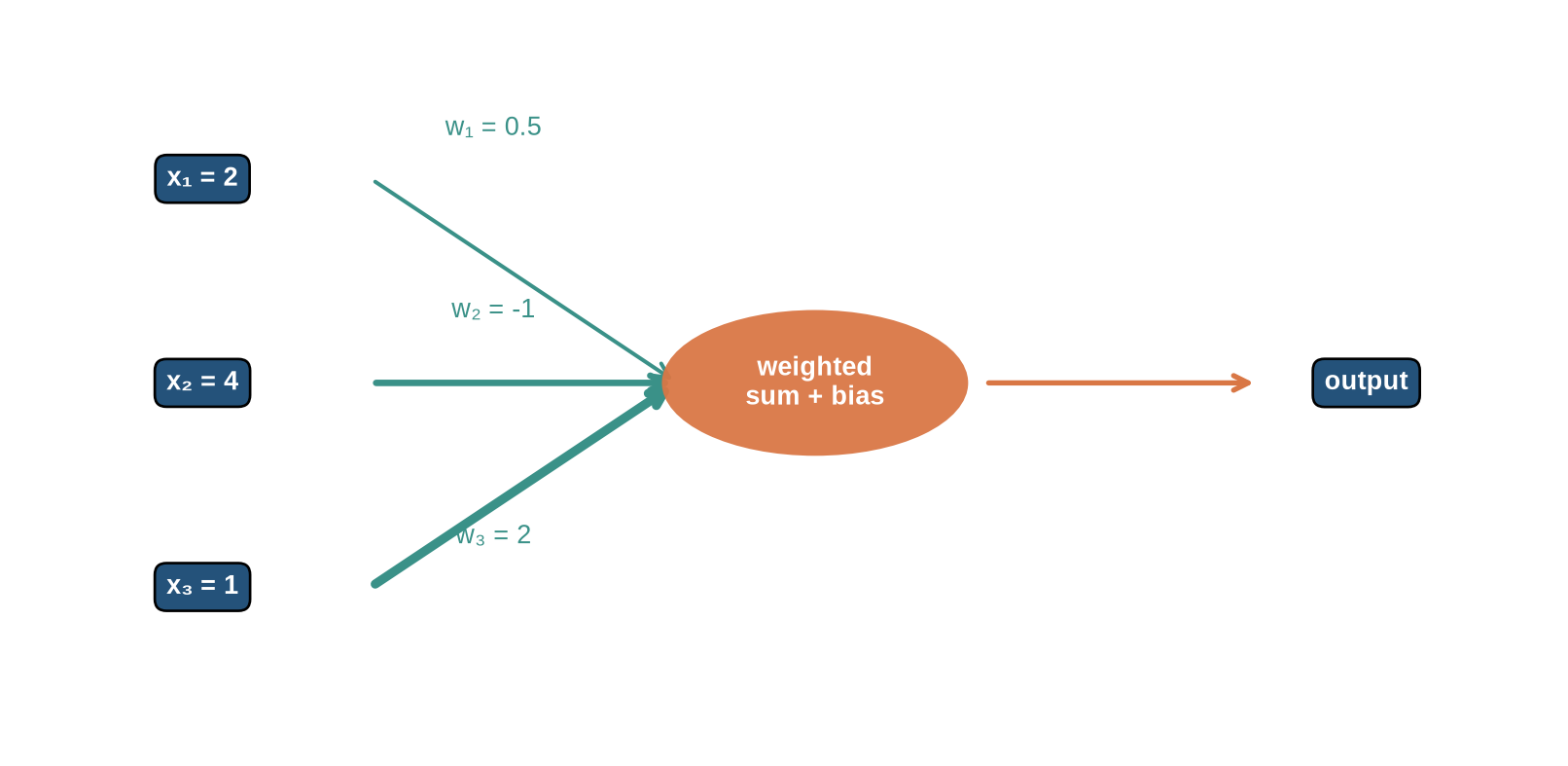
The diagram is an arithmetic recipe. Each incoming value is multiplied by the number written beside its arrow. The three products are added, the bias is included, and the total becomes the neuron's output.
### Inputs do not contribute equally
The weights allow the calculation to treat the inputs differently. A positive weight means that a larger input raises this neuron's score; a negative weight means that it lowers the score. A weight close to zero leaves little trace in this particular calculation. The signs and sizes are not chosen by hand in a trained network: they are adjusted from earlier examples.
```{python}
#| label: fig-neuron-intuition
#| fig-cap: "A neuron weights several inputs, combines them, and produces one output."
#| fig-alt: "Three input features with differently weighted arrows entering one neuron and producing an output."
import numpy as np
import matplotlib.pyplot as plt
from matplotlib.patches import Circle, FancyArrowPatch

plt.style.use("seaborn-v0_8-whitegrid")
blue, teal, orange, purple = "#24527a", "#3a9188", "#d97745", "#7655a6"

fig, ax = plt.subplots(figsize=(8.5, 4.2))
input_y = [0.78, 0.50, 0.22]
input_labels = ["x₁ = 2", "x₂ = 4", "x₃ = 1"]
weight_labels = ["w₁ = 0.5", "w₂ = -1", "w₃ = 2"]
weight_widths = [1.5, 2.5, 3.5]

for ypos, label, weight_label, width in zip(input_y, input_labels, weight_labels, weight_widths):
    ax.text(0.12, ypos, label, ha="center", va="center", color="white", weight="bold",
            bbox={"boxstyle": "round,pad=0.45", "facecolor": blue})
    ax.add_patch(FancyArrowPatch((0.23, ypos), (0.43, 0.5), arrowstyle="->",
                                 mutation_scale=14, linewidth=width, color=teal))
    ax.text(0.31, ypos + 0.06 if ypos != 0.5 else ypos + 0.09, weight_label,
            ha="center", color=teal)

ax.add_patch(Circle((0.52, 0.5), 0.10, facecolor=orange, alpha=0.95))
ax.text(0.52, 0.5, "weighted\nsum + bias", ha="center", va="center", color="white", weight="bold")
ax.add_patch(FancyArrowPatch((0.63, 0.5), (0.81, 0.5), arrowstyle="->",
                             mutation_scale=14, linewidth=2, color=orange))
ax.text(0.88, 0.5, "output", ha="center", va="center", color="white", weight="bold",
        bbox={"boxstyle": "round,pad=0.45", "facecolor": blue})
ax.set_xlim(0, 1); ax.set_ylim(0, 1); ax.axis("off")
plt.tight_layout()
plt.show()
```
The arrows encode the weights. The labels show why the three inputs do not have the same effect on the total: the second arrow has a negative weight, while the third has the largest positive weight.
::: {.concept-box .concept-core #concept-artificial-neuron data-term="Artificial neuron" data-domain="Foundations" data-symbols="x; w; b"}
**Artificial neuron.** A small calculation that gives each input a learned weight, adds the weighted inputs and a bias, and produces one value. An activation function may then transform that value before it is passed forward.
:::
### The bias sets a baseline
The bias is the part of the calculation that remains when all three inputs are zero. It moves the whole score up or down before any activation function is applied. Without it, the calculation would be forced through a particular starting point; with it, the model can learn where the score should sit before the inputs make their contributions.
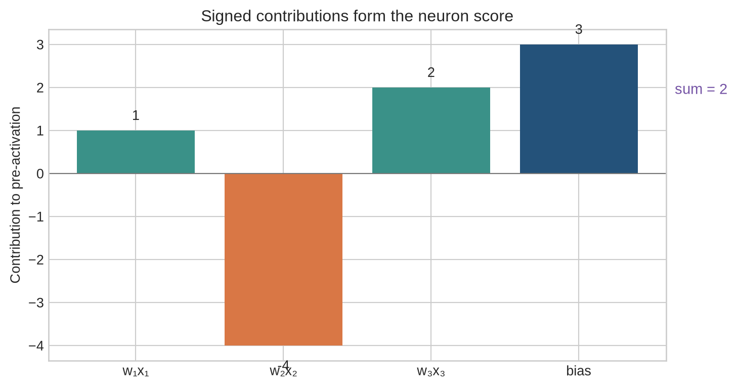
This is easiest to see after the arithmetic has been laid out. The three weighted contributions in the running example total $-1$. Adding the bias moves the total to $2$. The bias is therefore not an optional decoration: it is one of the quantities learned during training.
### Following the contributions
The arithmetic also explains why the largest input does not necessarily have the largest effect. Each input must be considered together with its weight.
```{python}
#| label: fig-weighted-contributions
#| fig-cap: "The neuron's pre-activation is the sum of signed weighted input contributions plus the bias; a large input does not necessarily make the largest contribution."
#| fig-alt: "A bar chart shows the three signed weighted contributions from the running example and the positive bias, followed by their summed pre-activation."
contribution_labels=["w₁x₁","w₂x₂","w₃x₃","bias"]
contribution_values=np.array([1.,-4.,2.,3.])
fig,ax=plt.subplots(figsize=(7.7,4.1))
bar_colours=[teal,orange,teal,blue]
ax.bar(contribution_labels,contribution_values,color=bar_colours)
for i,value in enumerate(contribution_values): ax.text(i,value+(.18 if value>=0 else -.34),f"{value:.0f}",ha="center",va="bottom" if value>=0 else "top")
ax.axhline(0,color="#777777",linewidth=.8); ax.text(3.65,1.85,"sum = 2",color=purple,fontsize=11)
ax.set(ylabel="Contribution to pre-activation",title="Signed contributions form the neuron score")
plt.tight_layout(); plt.show()
```
The second input is numerically largest, but its negative weight makes its contribution $-4$. The first input contributes $1$, the third contributes $2$, and the bias contributes $3$. Together they form the score $2$.
One neuron produces one number in this way. The next level follows the calculation line by line, then shows how the same rule is applied to many households at once.
## Level 2 - Mechanics
### Working through one neuron
Take the three inputs from the running example. First multiply each one by its corresponding weight. The table keeps the products separate before they are added:
| Input | Value $x_j$ | Weight $w_j$ | Contribution $w_jx_j$ |
|---|---:|---:|---:|
| $x_1$ | 2 | 0.5 | 1 |
| $x_2$ | 4 | -1 | -4 |
| $x_3$ | 1 | 2 | 2 |
They sum to $1-4+2=-1$. Adding the bias gives:
$$
z=-1+3=2.
$$
The number 2 is called the **pre-activation**, written $z$. It is the score before the neuron applies an activation function. If the activation is written $g$, the value passed onward is $a=g(z)$.
### How the bias changes a boundary
For two inputs and no activation, values with the same pre-activation satisfy:
$$
w_1x_1+w_2x_2+b=c.
$$
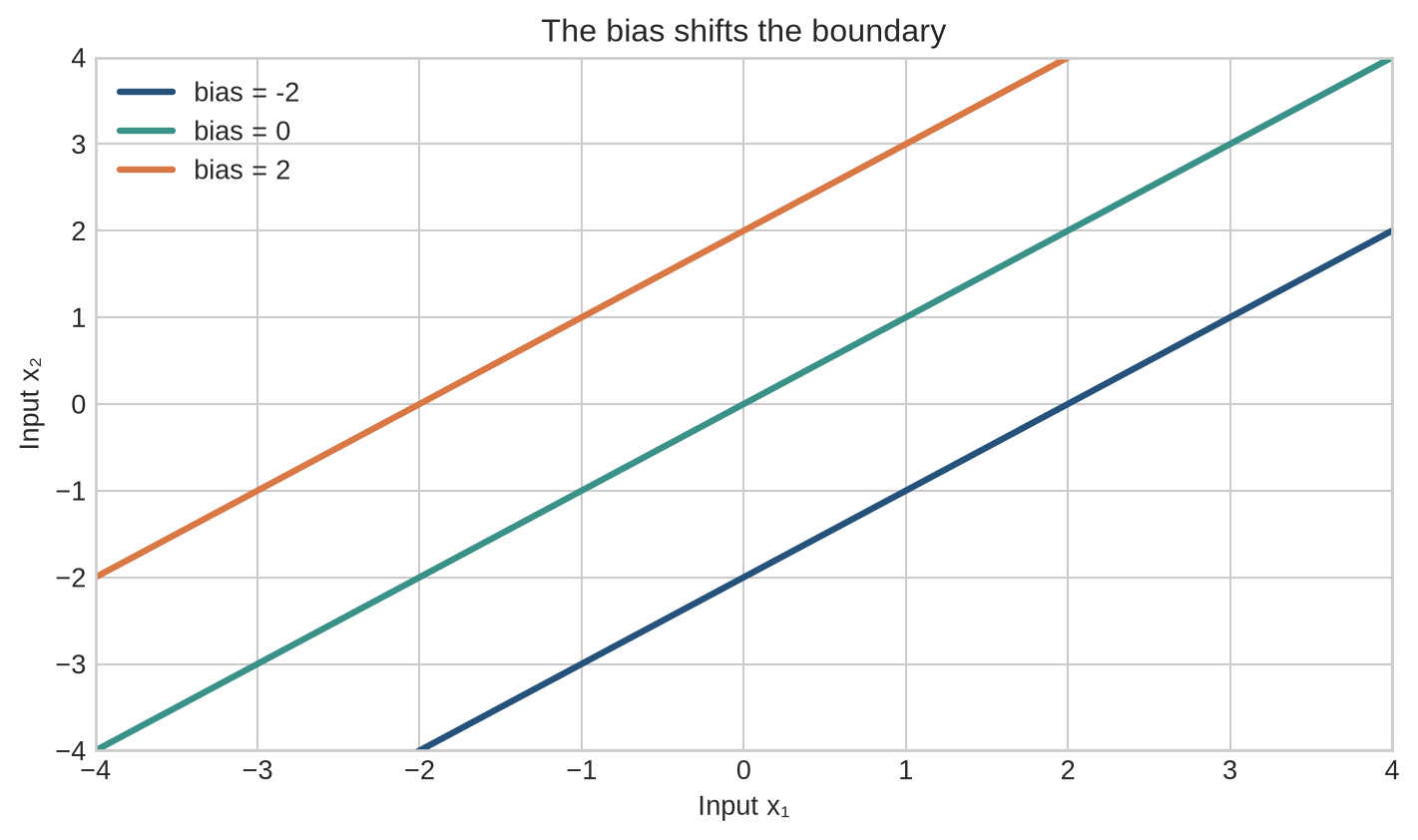
For a binary threshold at $z=0$, the decision boundary is $w_1x_1+w_2x_2+b=0$. Changing $b$ moves the boundary without changing its slope.
```{python}
#| label: fig-bias-boundary
#| fig-cap: "Changing the bias shifts a linear decision boundary while leaving its orientation unchanged."
#| fig-alt: "Three parallel decision boundaries corresponding to three bias values."
import numpy as np

x1 = np.linspace(-4, 4, 200)
w1, w2 = 1.0, -1.0
biases = [-2, 0, 2]
colours = [blue, teal, orange]

fig, ax = plt.subplots(figsize=(7.5, 4.5))
for bias, colour in zip(biases, colours):
    x2 = -(w1 * x1 + bias) / w2
    ax.plot(x1, x2, color=colour, linewidth=2.4, label=f"bias = {bias}")
ax.set(xlabel="Input x₁", ylabel="Input x₂", title="The bias shifts the boundary")
ax.set_xlim(-4, 4); ax.set_ylim(-4, 4)
ax.legend(frameon=False)
plt.tight_layout()
plt.show()
```
The three lines are parallel because the weights are unchanged. Their positions differ because the bias changes the score assigned to every point. This is why the bias is a learned parameter rather than a cosmetic addition.
### The activation changes what is passed forward
If the neuron uses the rectified linear unit, or ReLU,
$$
g(z)=\max(0,z),
$$
the running example produces $a=2$. A pre-activation of $-2$ would produce $a=0$. Different activation functions shape this hand-off in different ways; Chapter 7 examines that choice.
### A neuron during training
The forward pass calculates $z$ and $a$. The loss compares the eventual network output with the target. Backpropagation calculates gradients for the weight and bias, and the optimiser updates them. The inputs are data; the weights and bias are parameters. The activation function usually has a fixed form, although some architectures use activations with learned parameters.
The calculation is now complete for one household. The mathematics and code below express the same calculation compactly and then apply it to several households without changing the learned settings.
## Level 3 - Mathematics & Code
The mechanics can now be written compactly. This level introduces each symbol, checks the arithmetic manually, implements the same operation in PyTorch, and shows why nonlinearity is required between layers.
### Vector form
Let $x\in\mathbb{R}^p$ contain $p$ input features, $w\in\mathbb{R}^p$ contain one weight for each feature, and $b\in\mathbb{R}$ be a scalar bias. The neuron computes:
$$
z=w^\top x+b=\sum_{j=1}^{p}w_jx_j+b,
$$
followed by:
$$
a=g(z).
$$
The transpose in $w^\top x$ turns the two vectors into a dot product. Each pair $w_jx_j$ produces one contribution; the sum and bias produce one scalar $z$; the activation converts that scalar into the value sent to the next layer.
For the running example:
$$
z=0.5(2)+(-1)(4)+2(1)+3=2.
$$
```{python}
import torch

x = torch.tensor([2.0, 4.0, 1.0])
w = torch.tensor([0.5, -1.0, 2.0])
b = torch.tensor(3.0)

contributions = w * x
z = torch.dot(w, x) + b
a = torch.relu(z)

print("weighted contributions:", contributions)
print(f"pre-activation z: {z.item():.1f}")
print(f"ReLU activation a: {a.item():.1f}")
```
The code exposes the same stages as the table in Level 2. Elementwise multiplication produces the three contributions. `torch.dot` sums them. Adding `b` produces the pre-activation, and `torch.relu` applies the activation.
### Manual parameters and `nn.Linear`
PyTorch's `Linear` layer implements the affine transformation. Its stored weight uses shape `(out_features, in_features)`, so a one-output layer with three inputs has a weight matrix of shape `(1, 3)` and one bias.
```{python}
import torch.nn as nn

layer = nn.Linear(3, 1)
with torch.no_grad():
    layer.weight.copy_(w.reshape(1, 3))
    layer.bias.copy_(b.reshape(1))

layer_output = layer(x)
print("weight shape:", tuple(layer.weight.shape))
print("bias shape:", tuple(layer.bias.shape))
print(f"layer output: {layer_output.item():.1f}")
```
The result equals the manual pre-activation because both calculations use the same parameters. `nn.Linear` does not apply ReLU automatically. Keeping the affine transformation and activation separate allows architectures to choose different activation functions.
The stored orientation is worth checking because it prevents a common shape error. A one-neuron layer stores one row of weights, so `layer.weight` has shape $(1,3)$. A batch with shape $(B,3)$ returns an affine output with shape $(B,1)$. The extra final axis represents one output feature per observation; it should not be removed accidentally when later code expects a feature dimension.
### Applying one neuron to a batch
The running calculation used one input vector and produced one output. In code, the same weight vector and bias are applied to every row in a batch. A batch of shape $B\times p$ therefore produces one pre-activation and one activation for each of its $B$ observations; the number of learned parameters does not grow with the batch.
```{python}
batch=np.array([[2.,4.,1.],[0.,1.,3.],[-1.,2.,2.]])
weights=np.array([.5,-1.,2.]); bias=3.
batch_z=batch@weights+bias
batch_a=np.maximum(0,batch_z)
print("input batch shape:",batch.shape)
print("shared weight and bias shapes:",weights.shape,np.asarray(bias).shape)
print("pre-activations:",batch_z)
print("ReLU activations:",batch_a)
```
The three outputs belong to three observations, not to three different neurons. Chapter 6 adds multiple learned weight vectors to produce several outputs for each observation.
### Activation functions
```{python}
#| label: fig-activation-functions
#| fig-cap: "Activation functions transform the pre-activation in different ways."
#| fig-alt: "Plots of sigmoid, tanh, ReLU, and GELU across pre-activation values from minus five to five."
z_values = torch.linspace(-5, 5, 400)
activations = {
    "Sigmoid": torch.sigmoid(z_values),
    "Tanh": torch.tanh(z_values),
    "ReLU": torch.relu(z_values),
    "GELU": torch.nn.functional.gelu(z_values),
}

fig, axes = plt.subplots(2, 2, figsize=(9, 6), sharex=True)
for ax, (name, values), colour in zip(axes.flat, activations.items(), [blue, teal, orange, blue]):
    ax.plot(z_values.numpy(), values.numpy(), color=colour, linewidth=2.4)
    ax.axhline(0, color="#777777", linewidth=0.7)
    ax.axvline(0, color="#777777", linewidth=0.7)
    ax.set_title(name)
    ax.set_ylabel("Activation")
for ax in axes[1]:
    ax.set_xlabel("Pre-activation z")
plt.tight_layout()
plt.show()
```
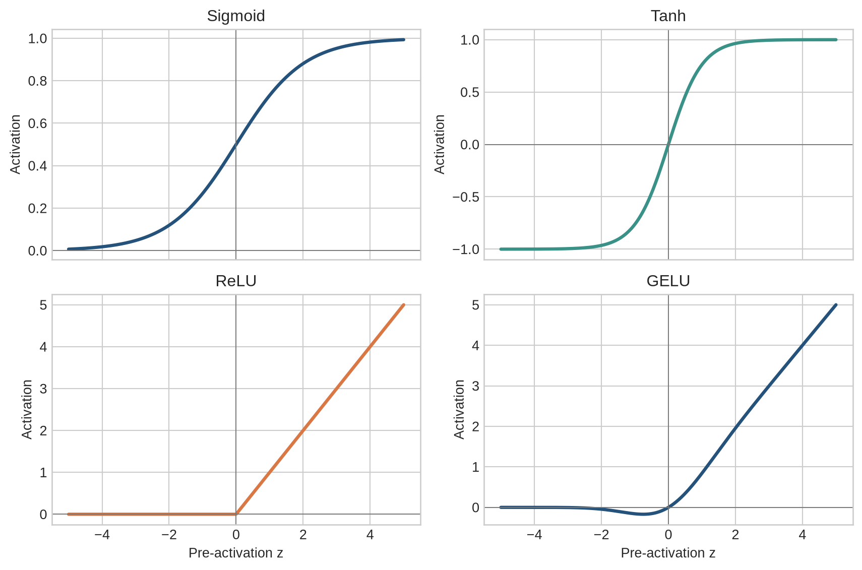
Sigmoid maps values to $(0,1)$ and is useful when an output is interpreted as a binary probability. Tanh maps to $(-1,1)$. ReLU sets negative values to zero and leaves positive values unchanged. GELU changes values smoothly according to their magnitude and is widely used in Transformer feed-forward blocks [@hendrycks2016gelu]. The choice affects representation, gradients, and numerical behaviour.
### Why stacked linear layers are still linear
Suppose two layers omit their activations:
$$
h=W_1x+b_1,
$$
$$
y=W_2h+b_2.
$$
Substituting the first equation into the second gives:
$$
y=W_2W_1x+(W_2b_1+b_2).
$$
This has the same affine form as one layer. Depth alone therefore does not create nonlinear representational capacity. The activation between layers prevents the composition from collapsing into one affine transformation.
The argument concerns the function represented by the composition, not the usefulness of intermediate dimensions for every computational purpose. Two affine operations may be implemented separately for engineering or parameter-sharing reasons, but they do not introduce an input-dependent bend in the input-output mapping until a nonlinearity intervenes. Chapter 7 examines those bends and their derivatives directly.
## Level 4 - Research & Systems
Chapter 6 develops the move from one neuron to a layer. Here the question is different: what changes when the same weighted-sum calculation is executed at the scale of contemporary models? The relevant constraints are matrix shapes, stored activations, memory traffic, numerical precision, and the need to initialise many units differently.
### Feed-forward blocks in Transformers
A Transformer feed-forward block applies two learned projections with an activation between them [@vaswani2017]:
$$
\operatorname{FFN}(x)=W_2g(W_1x+b_1)+b_2.
$$
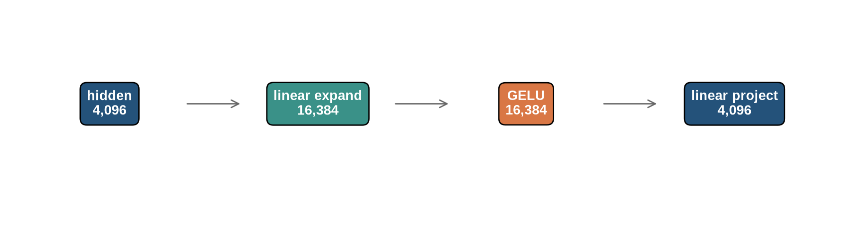
The first projection usually expands the hidden dimension; the second projects it back. If the hidden width is 4,096 and the intermediate width is 16,384, the first weight matrix alone contains $4{,}096\times16{,}384=67{,}108{,}864$ parameters. The operation is conceptually a layer of many artificial neurons, but its systems behaviour is governed by matrix shapes, memory traffic, and accelerator kernels.
```{python}
#| label: fig-transformer-ffn
#| fig-cap: "A Transformer feed-forward block expands, activates, and projects each token representation."
#| fig-alt: "A flow diagram from hidden representation through expansion, GELU activation, and projection back to the hidden width."
fig, ax = plt.subplots(figsize=(9, 2.5))
blocks = [
    (0.12, "hidden\n4,096", blue),
    (0.37, "linear expand\n16,384", teal),
    (0.62, "GELU\n16,384", orange),
    (0.87, "linear project\n4,096", blue),
]
for xpos, label, colour in blocks:
    ax.text(xpos, 0.55, label, ha="center", va="center", color="white", weight="bold",
            bbox={"boxstyle": "round,pad=0.5", "facecolor": colour})
for left, right in zip(blocks[:-1], blocks[1:]):
    ax.add_patch(FancyArrowPatch((left[0] + 0.09, 0.55), (right[0] - 0.09, 0.55),
                                 arrowstyle="->", mutation_scale=14, color="#666666"))
ax.set_xlim(0, 1); ax.set_ylim(0, 1); ax.axis("off")
plt.tight_layout()
plt.show()
```
The figure represents one token position, but implementations process many token positions and sequences together. The same weight matrices are applied across those positions. This reuse distinguishes the feed-forward block from attention, which mixes information across token positions.
### Initialisation, scale, and gradient flow
Weights cannot all start at the same value because units would receive identical gradients and remain symmetric. They are usually sampled from distributions whose scale depends on layer width. Poorly scaled initialisation can make activations and gradients grow, vanish, or saturate as they pass through many layers. Xavier/Glorot initialisation was developed to control this behaviour for particular activation assumptions [@glorot2010].
Training then changes the weights using the gradients developed in [Chapter 3](03-gradient-descent.qmd) and [Chapter 4](04-backpropagation.qmd). The neuron equation remains the forward computation; backpropagation supplies $\partial L/\partial W$ and $\partial L/\partial b$ for the whole layer.
Symmetry explains why identical initial weights are unsuitable for a layer with several units. If two units begin with identical weights and biases and receive the same inputs, they produce identical outputs and receive identical gradients under the same downstream path. Updating them preserves the duplication. Random initialisation gives the units different starting directions; the training signal can then differentiate their roles if the data and objective support it.
### Hardware and numerical precision
Large linear layers are often limited by the rate at which hardware can move weights and activations as well as by arithmetic throughput. Lower-precision formats reduce memory and can increase matrix-multiplication throughput, but training must retain sufficient numerical range for gradients and optimiser state [@micikevicius2018]. Kernel fusion can reduce the movement of intermediate values by combining bias addition and activation with the matrix multiplication.
These systems choices do not alter the definition of a neuron. They determine how millions of neuron-equivalent operations are represented and executed efficiently.
The same distinction applies to parameter precision. A model may store some values in lower precision for throughput while retaining selected accumulators or optimiser state at higher precision. Reporting only that a network uses an activation or a linear layer says little about the numerical contract under which it was trained. Chapter 8 assembles these choices into a training loop; Chapters 11-15 examine their optimisation and systems consequences.
## Common misconceptions
- **An artificial neuron behaves like a biological neuron.** The terminology is historical; the artificial neuron is a parameterised mathematical operation.
- **A neuron makes an intelligent decision.** It calculates a weighted sum, adds a bias, and applies an activation.
- **A weight is automatically a causal effect or feature importance.** It is a fitted parameter whose meaning depends on scaling, other parameters, and the model architecture.
- **The bias is optional in principle and therefore unimportant.** Some architectures omit biases, but when present the bias changes the affine transformation and is trained with the weights.
- **`nn.Linear` includes an activation.** It performs the affine transformation only; the activation is a separate operation.
- **Stacking linear layers creates a nonlinear model.** Without activations, their composition is another affine transformation.
- **Transformers simulate neurons individually.** Implementations use batched tensor and matrix operations.
## Exercises
1. For $x=(3,2)$, $w=(2,-1)$, and $b=1$, calculate the weighted contributions and pre-activation.
2. Apply ReLU to the result of Exercise 1.
3. Explain how changing the bias affects a two-dimensional linear decision boundary.
4. Why should a fitted weight not automatically be interpreted as a causal effect?
5. Write the tensor shapes for a batch of 64 observations, 128 input features, and 512 output units.
6. Calculate the number of parameters in the layer from Exercise 5, including biases.
7. Implement the running example with `nn.Linear` and verify that it matches the manual calculation.
8. Explain why two linear layers without an activation can be replaced by one linear layer.
9. Compare ReLU and GELU using the activation plot. What happens for negative pre-activations?
10. A feed-forward block expands width 1,024 to 4,096 and projects it back. Calculate the number of weight parameters, excluding biases.
11. Why can activation and weight scale affect gradient flow?
12. Explain why a GPU implementation uses matrix multiplication rather than a loop over neuron objects.
13. Calculate the pre-activation and ReLU output for each row of the batch introduced in Level 2.
14. Explain why a batch of 100 observations does not give a one-neuron layer 100 sets of learned weights.
15. State the input, weight, bias, and output shapes for a one-output `nn.Linear` layer applied to a batch of shape $(32,3)$.
16. Explain why two units that start with identical weights and biases can remain redundant during training.
## Summary
An artificial neuron calculates an affine transformation $z=w^\top x+b$ and usually applies an activation $a=g(z)$. Weights control input contributions, while the bias shifts the transformation. Activation functions prevent stacked layers from collapsing into one affine function. Modern neural networks execute many neuron-equivalent operations as batched matrix multiplications. Transformer feed-forward blocks use the same structure at a much larger scale: projection, activation, and projection back.
## Looking ahead
One neuron produces one scalar activation. A neural-network layer produces a vector, and successive layers build increasingly complex representations. [Chapter 6](06-neural-network-layers.qmd) develops layer dimensions, matrix operations, and composition. [Chapter 7](07-activation-functions.qmd) then examines activation functions and non-linearity in greater depth.
## Further reading
Early formal treatments of artificial neural units include @mcculloch1943 and @rosenblatt1958. The role of initialisation in deep networks is examined by @glorot2010. GELU is introduced by @hendrycks2016gelu, and the Transformer feed-forward architecture is described by @vaswani2017.