---
title: "Building a Small Neural Network"
subtitle: "From data to updated predictions"
---
## The problem
Chapters 1–7 introduced the parts of a neural network separately. We now have data, layers, activations, a loss, a way to calculate gradients, and an optimiser. None of those parts learns on its own. They must be connected in an order that lets an earlier prediction change the parameters used for the next one.
This chapter joins them in one small binary classifier. The data are deliberately simple: two curved groups that one straight boundary cannot separate. They make the training sequence visible before the book turns to the harder question of whether a fitted model will work beyond the records used to train it.
### The data boundary
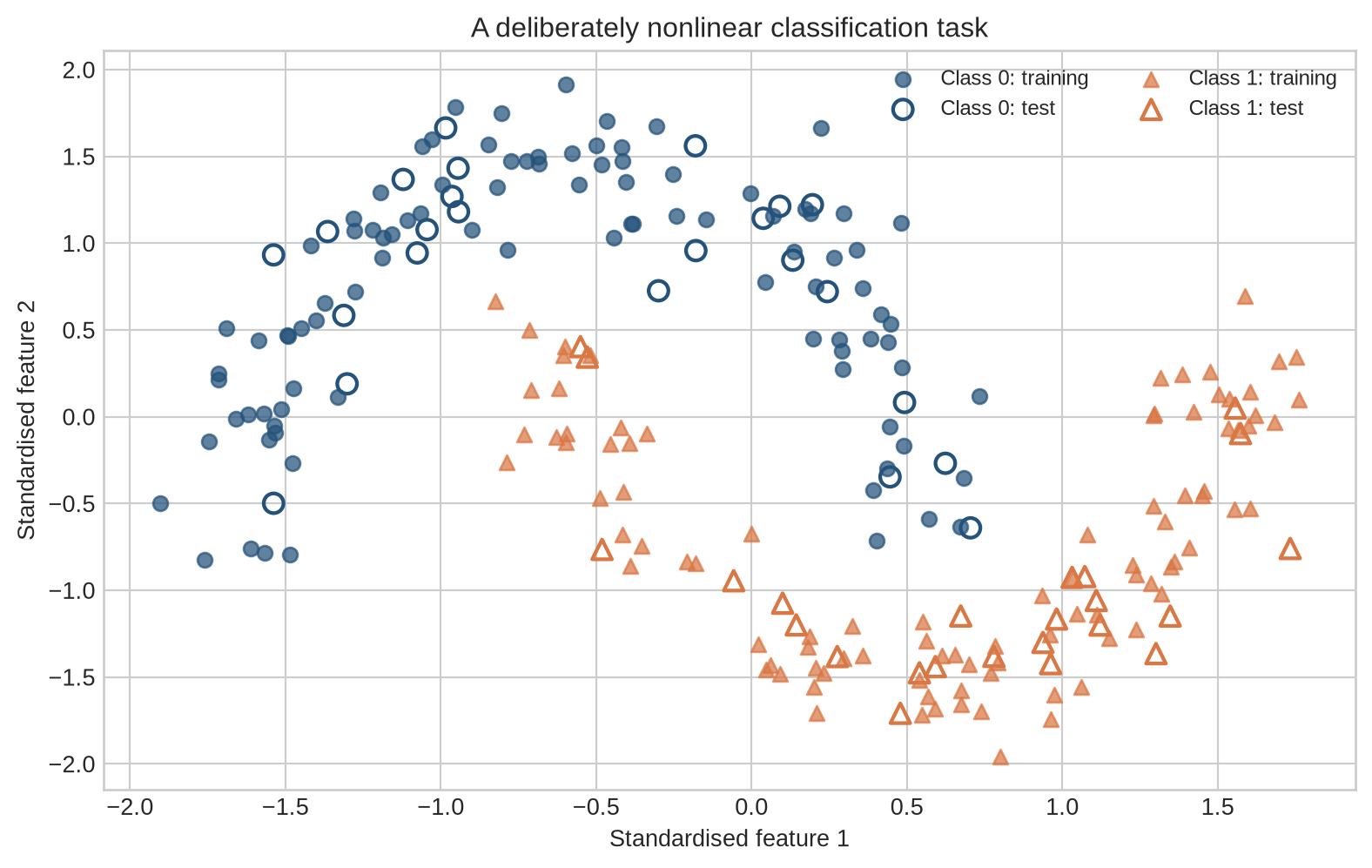
The dataset contains 240 two-dimensional observations arranged as two noisy interlocking curves. The label indicates which curve generated an observation. The training set contains 192 observations and the test set contains 48. Input standardisation uses the training-set mean and standard deviation; test-set information is not used to define the transformation.
Before looking at the training loop, inspect the data. The two curves are deliberately arranged so that one straight line cannot separate them. Outlined observations are held out from fitting, so they can later show whether the learned boundary extends beyond the examples used for updates.
```{python}
#| label: fig-small-network-data
#| fig-cap: "The synthetic task contains two classes with a curved boundary; colour shows the label and marker shape shows the data split."
#| fig-alt: "A scatter plot shows two noisy interlocking curves. Blue circles and orange triangles represent the two classes, with outlined markers identifying test observations."
import numpy as np
import matplotlib.pyplot as plt
from matplotlib.patches import FancyBboxPatch, FancyArrowPatch

plt.style.use("seaborn-v0_8-whitegrid")
blue, teal, orange, purple, grey = "#24527a", "#3a9188", "#d97745", "#7a5195", "#5f6b76"
rng = np.random.default_rng(27)
n_per_class = 120
theta0 = rng.uniform(0, np.pi, n_per_class)
theta1 = rng.uniform(0, np.pi, n_per_class)
x0 = np.column_stack([np.cos(theta0), np.sin(theta0)])
x1 = np.column_stack([1 - np.cos(theta1), 0.45 - np.sin(theta1)])
X_raw = np.vstack([x0, x1]) + rng.normal(0, 0.11, size=(2 * n_per_class, 2))
y_raw = np.concatenate([np.zeros(n_per_class), np.ones(n_per_class)])

train_indices, test_indices = [], []
for class_value in [0, 1]:
    class_indices = np.flatnonzero(y_raw == class_value)
    rng.shuffle(class_indices)
    train_indices.extend(class_indices[:96])
    test_indices.extend(class_indices[96:])
train_indices, test_indices = np.array(train_indices), np.array(test_indices)
rng.shuffle(train_indices); rng.shuffle(test_indices)
X_train_raw, y_train_np = X_raw[train_indices], y_raw[train_indices]
X_test_raw, y_test_np = X_raw[test_indices], y_raw[test_indices]
train_mean, train_std = X_train_raw.mean(axis=0), X_train_raw.std(axis=0)
X_train_np = (X_train_raw - train_mean) / train_std
X_test_np = (X_test_raw - train_mean) / train_std

fig, ax = plt.subplots(figsize=(8.3, 5.3))
for class_value, colour, marker in [(0, blue, "o"), (1, orange, "^")]:
    train_mask, test_mask = y_train_np == class_value, y_test_np == class_value
    ax.scatter(X_train_np[train_mask, 0], X_train_np[train_mask, 1], c=colour,
               marker=marker, s=40, alpha=0.72, label=f"Class {class_value}: training")
    ax.scatter(X_test_np[test_mask, 0], X_test_np[test_mask, 1], facecolors="none",
               edgecolors=colour, marker=marker, s=72, linewidths=1.6,
               label=f"Class {class_value}: test")
ax.set_xlabel("Standardised feature 1"); ax.set_ylabel("Standardised feature 2")
ax.set_title("A deliberately nonlinear classification task")
ax.legend(ncol=2, fontsize=9)
plt.tight_layout(); plt.show()
```
The outlined observations remain outside training. They let us see whether the final boundary extends to records that did not contribute to the updates. The split is for this illustration; Chapter 9 develops the evidence required to assess generalisation.
## Level 1 - Intuition
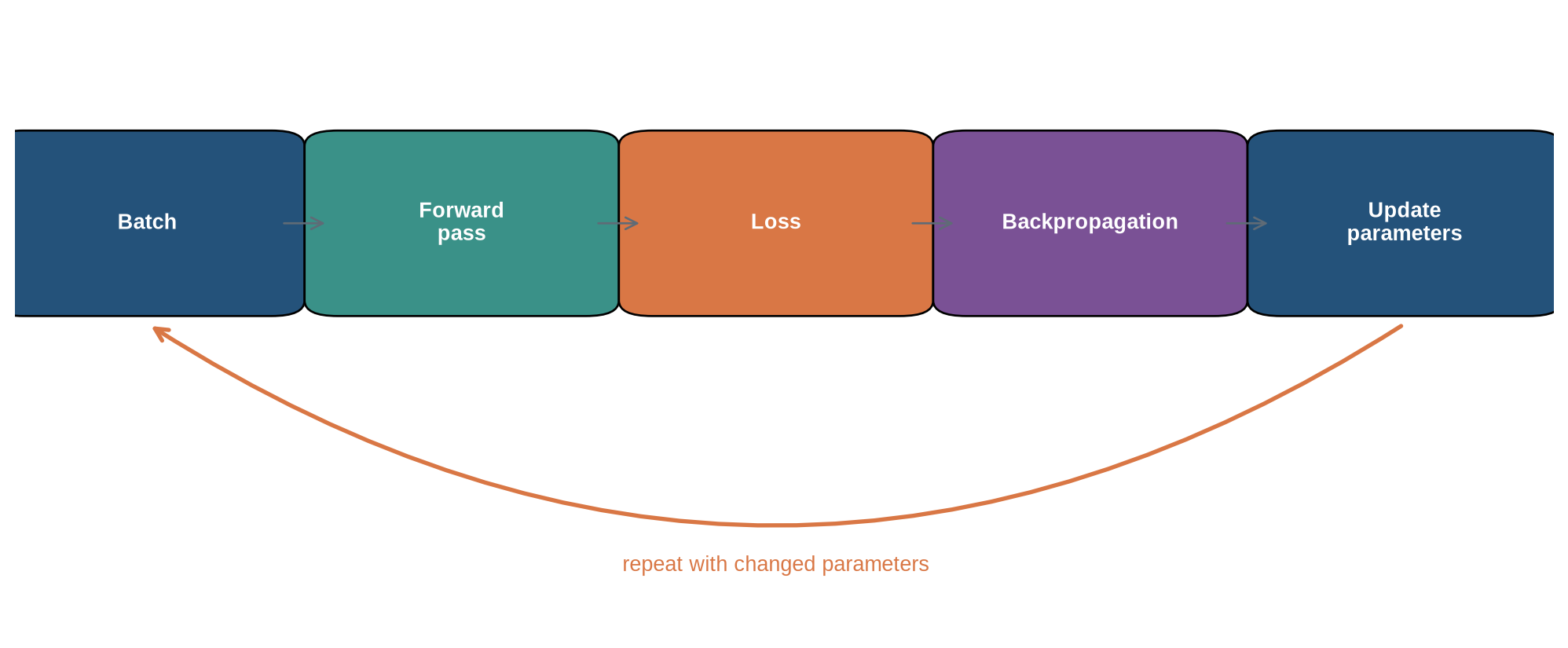
The training loop is where the earlier chapters become one procedure. Follow one cycle before reading the implementation: take a batch, calculate scores, compare them with the recorded outcomes, send the resulting information backwards, and change the weights used for the next batch.
### Training is a repeated comparison followed by a correction
A neural network begins with parameter values that do not yet encode the pattern in the data. It processes a batch and produces predictions. The loss measures the disagreement between those predictions and the labels. Backpropagation attributes part of that loss to each parameter, and the optimiser makes a small update intended to reduce future loss.
The update does not edit a prediction directly. It changes weights and biases. Every later prediction is recalculated through the revised network. Learning is the accumulated result of many such updates.
```{python}
#| label: fig-training-loop-intuition
#| fig-cap: "A training loop connects a batch, forward pass, loss, backpropagation, and parameter update before processing the next batch."
#| fig-alt: "Five rounded boxes form a loop: batch, forward pass, loss, backpropagation, and update. An arrow returns from the update to the next batch."
fig, ax = plt.subplots(figsize=(10.5, 4.4))
steps = [(0.08,"Batch",blue),(0.27,"Forward\npass",teal),(0.46,"Loss",orange),
         (0.65,"Backpropagation",purple),(0.84,"Update\nparameters",blue)]
for xpos, label, colour in steps:
    box = FancyBboxPatch((xpos-0.075,0.48),0.15,0.20,boxstyle="round,pad=0.02",
                         facecolor=colour,edgecolor="black",linewidth=1.0)
    ax.add_patch(box); ax.text(xpos,0.58,label,ha="center",va="center",color="white",weight="bold")
for left, right in zip(steps[:-1], steps[1:]):
    ax.add_patch(FancyArrowPatch((left[0]+0.08,0.58),(right[0]-0.08,0.58),
                                 arrowstyle="->",mutation_scale=14,color=grey))
ax.add_patch(FancyArrowPatch((0.84,0.45),(0.08,0.45),connectionstyle="arc3,rad=-0.32",
                             arrowstyle="->",mutation_scale=15,color=orange,linewidth=2))
ax.text(0.46,0.13,"repeat with changed parameters",ha="center",color=orange)
ax.set_xlim(0,0.93); ax.set_ylim(0.05,0.85); ax.axis("off")
plt.tight_layout(); plt.show()
```
Each box has one role. The batch supplies inputs and recorded outcomes. The forward pass produces scores. The loss compares those scores with the outcomes. Backpropagation calculates how each parameter contributed to that loss, and the optimiser changes the parameters. Reversing these dependencies would change the algorithm.
::: {.concept-box .concept-core #concept-training-loop data-term="Training loop" data-domain="Foundations"}
**Training loop.** The repeated sequence that takes a batch, makes predictions, calculates their loss, traces gradients backwards, and updates the model's parameters.
:::
### The network creates a boundary by combining simple transformations
The model used here has two input features, sixteen hidden units with tanh activations, and one output logit. Each hidden unit creates one transformed view of the input. The output layer combines those sixteen values. Because tanh is nonlinear, the resulting boundary can bend around the interlocking classes.
The final layer produces one score. In the next level, that score will be converted into a probability and compared with the known class. For now, the important point is that the network can bend its boundary because the hidden layer uses a non-linear activation.
Level 2 follows one observation through the operations that the loop repeats.
## Level 2 - Mechanics
### One observation moves forward through six calculations
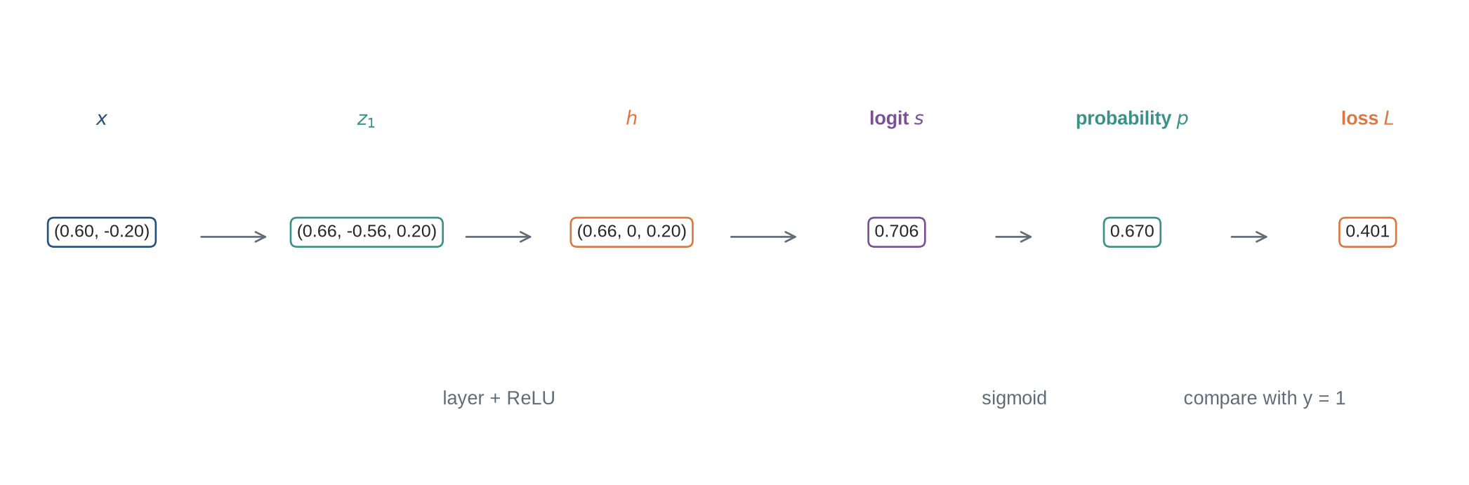
To keep the arithmetic visible, use a smaller network with two inputs, three hidden units, and one output. For $x=(0.6,-0.2)$, let
$$
W_1=\begin{bmatrix}0.8&-0.4\\-0.3&0.9\\0.5&0.5\end{bmatrix},\qquad
b_1=(0.1,-0.2,0).
$$
The first pre-activation is $z_1=W_1x+b_1=(0.66,-0.56,0.20)$. ReLU gives $h=(0.66,0,0.20)$. With output weights $W_2=(1.1,-0.7,0.4)$ and bias $b_2=-0.1$, the logit is $s=W_2h+b_2=0.706$. Sigmoid converts it to $p=0.670$. If $y=1$, binary cross-entropy is $L=-\log(p)=0.401$.
The model assigns more probability to the correct class than to the alternative, but the loss remains positive because the predicted probability is below one.
```{python}
#| label: fig-one-observation-forward
#| fig-cap: "One observation becomes hidden pre-activations, activated values, a logit, a probability, and finally a loss."
#| fig-alt: "A horizontal sequence shows input x, first-layer pre-activation z, ReLU hidden values h, logit s, probability p, and binary cross-entropy loss L with their numerical values."
fig, ax = plt.subplots(figsize=(11,3.7))
items=[(0.06,r"$x$","(0.60, -0.20)",blue),(0.24,r"$z_1$","(0.66, -0.56, 0.20)",teal),
       (0.42,r"$h$","(0.66, 0, 0.20)",orange),(0.60,r"logit $s$","0.706",purple),
       (0.76,r"probability $p$","0.670",teal),(0.92,r"loss $L$","0.401",orange)]
for xpos, heading, value, colour in items:
    ax.text(xpos,0.62,heading,ha="center",weight="bold",color=colour)
    ax.text(xpos,0.42,value,ha="center",fontsize=9.5,
            bbox={"boxstyle":"round,pad=0.35","facecolor":"white","edgecolor":colour})
for left,right in zip(items[:-1],items[1:]):
    ax.add_patch(FancyArrowPatch((left[0]+0.065,0.42),(right[0]-0.065,0.42),
                                 arrowstyle="->",mutation_scale=13,color=grey))
ax.text(0.33,0.12,"layer + ReLU",ha="center",color=grey)
ax.text(0.68,0.12,"sigmoid",ha="center",color=grey)
ax.text(0.85,0.12,"compare with y = 1",ha="center",color=grey)
ax.set_xlim(0,0.98); ax.set_ylim(0,0.82); ax.axis("off")
plt.tight_layout(); plt.show()
```
The intermediate values make errors diagnosable. A wrong shape appears at the layer calculation. An unexpected zero appears after ReLU. A probability outside $(0,1)$ indicates that sigmoid was omitted or misapplied. A non-scalar per-observation loss may indicate that reduction has not yet been performed.
### Backpropagation reverses the dependency chain
For sigmoid combined with binary cross-entropy,
$$
\delta_s=\frac{\partial L}{\partial s}=p-y=0.670-1=-0.330.
$$
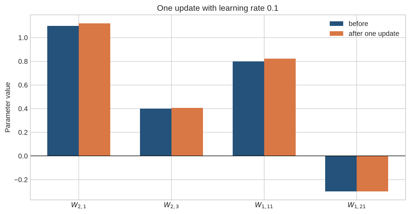
The negative sign says that increasing the logit would reduce the loss for this positive-labelled observation. The output-weight gradient is $\delta_s h$, and the output-bias gradient is $\delta_s$. The gradient arriving at the hidden activations is $W_2^\top\delta_s$.
ReLU blocks the gradient through the second hidden unit because its pre-activation was negative. The other two units pass their gradients. The same chain rule used in Chapter 4 therefore produces gradients for every parameter in both layers.
```{python}
#| label: fig-one-step-update
#| fig-cap: "A gradient-descent update moves selected parameters in the direction that lowers the current observation's loss."
#| fig-alt: "A paired bar chart compares four representative parameter values before and after one update, showing small changes and no change for a weight feeding the inactive hidden unit."
p_example=1/(1+np.exp(-0.706)); delta_s=p_example-1
h_example=np.array([0.66,0.0,0.20]); x_example=np.array([0.6,-0.2])
w2_example=np.array([1.1,-0.7,0.4]); z_example=np.array([0.66,-0.56,0.20])
delta_z=(w2_example*delta_s)*(z_example>0)
grad_w1=np.outer(delta_z,x_example); grad_w2=delta_s*h_example; learning_rate=0.1
before=np.array([1.1,0.4,0.8,-0.3])
after=np.array([1.1-learning_rate*grad_w2[0],0.4-learning_rate*grad_w2[2],
                0.8-learning_rate*grad_w1[0,0],-0.3-learning_rate*grad_w1[1,0]])
labels=[r"$W_{2,1}$",r"$W_{2,3}$",r"$W_{1,11}$",r"$W_{1,21}$"]
positions=np.arange(len(labels)); width=0.34
fig,ax=plt.subplots(figsize=(8.5,4.5))
ax.bar(positions-width/2,before,width,label="before",color=blue)
ax.bar(positions+width/2,after,width,label="after one update",color=orange)
ax.axhline(0,color="black",linewidth=0.8); ax.set_xticks(positions,labels)
ax.set_ylabel("Parameter value"); ax.set_title("One update with learning rate 0.1"); ax.legend()
plt.tight_layout(); plt.show()
```
The changes are intentionally small. The fourth parameter feeds the inactive second hidden unit, so its gradient is zero for this observation and its bar does not move. A batch can produce a non-zero gradient for the same parameter if other observations activate that unit.
## Level 3 - Mathematics & Code
Level 2 followed one observation through one update. Actual code carries out the same chain for a batch, keeps gradients and optimiser state separately, and evaluates the trained model without changing it.
### A mini-batch loop repeats four actions
For each batch, an implementation normally clears stored gradients, runs the forward pass and loss, runs backpropagation, and asks the optimiser to update the parameters. PyTorch accumulates gradients by default. Omitting the clearing step therefore adds the current batch gradient to gradients already stored on each parameter. Gradient accumulation can be deliberate when several micro-batches should form one larger effective batch. Without that intention, it changes the update rule.
### Evaluation uses the model without parameter updates
Evaluation requires no backward pass or optimiser step. The model should be placed in evaluation mode because dropout and batch normalisation behave differently during training. Gradient tracking should also be disabled to reduce memory use. This network contains neither dropout nor batch normalisation, but using the correct pattern prevents errors when the architecture changes.
### The batch equations define the complete model
For $X\in\mathbb{R}^{B\times2}$, hidden width $H=16$, and $y\in\{0,1\}^B$,
$$
\begin{aligned}
Z_1 &= XW_1^\top+b_1, & W_1&\in\mathbb{R}^{16\times2},\\
H_1 &= \tanh(Z_1), & H_1&\in\mathbb{R}^{B\times16},\\
s &= H_1W_2^\top+b_2, & W_2&\in\mathbb{R}^{1\times16},\\
p &= \sigma(s).&&
\end{aligned}
$$
The batch-mean binary cross-entropy is
$$
L=-\frac{1}{B}\sum_{i=1}^{B}[y_i\log p_i+(1-y_i)\log(1-p_i)].
$$
In code, `BCEWithLogitsLoss` receives $s$ and $y$ and combines sigmoid with cross-entropy. This avoids explicitly calculating logarithms of probabilities that may round to zero or one.
### One manual NumPy step exposes every gradient
```{python}
x=np.array([0.6,-0.2]); y=1.0
W1=np.array([[0.8,-0.4],[-0.3,0.9],[0.5,0.5]]); b1=np.array([0.1,-0.2,0.0])
W2=np.array([[1.1,-0.7,0.4]]); b2=np.array([-0.1])
z1=W1@x+b1; h1=np.maximum(0,z1); logit=(W2@h1+b2).item()
probability=1/(1+np.exp(-logit))
loss=-(y*np.log(probability)+(1-y)*np.log(1-probability))
ds=probability-y; dW2=ds*h1[None,:]; db2=np.array([ds])
dh1=W2.ravel()*ds; dz1=dh1*(z1>0); dW1=np.outer(dz1,x); db1=dz1
print("z1:",np.round(z1,3)); print("h1:",np.round(h1,3))
print("logit, probability, loss:",np.round([logit,probability,loss],3))
print("dW2:",np.round(dW2,3)); print("dW1:\n",np.round(dW1,3))
```
The second row of `dW1` is zero because the second hidden unit is inactive. The remaining gradients match the dependency chain described in Level 2. A vectorised batch implementation replaces outer products with matrix multiplications and averages or sums gradients according to the loss reduction.
### PyTorch separates model, loss, and optimiser
```{python}
import torch
from torch import nn

torch.manual_seed(27)
X_train=torch.tensor(X_train_np,dtype=torch.float32)
y_train=torch.tensor(y_train_np,dtype=torch.float32).unsqueeze(1)
X_test=torch.tensor(X_test_np,dtype=torch.float32)
y_test=torch.tensor(y_test_np,dtype=torch.float32).unsqueeze(1)
model=nn.Sequential(nn.Linear(2,16),nn.Tanh(),nn.Linear(16,1))
loss_function=nn.BCEWithLogitsLoss()
optimiser=torch.optim.Adam(model.parameters(),lr=0.03)
parameter_count=sum(parameter.numel() for parameter in model.parameters())
print(model); print("Trainable parameters:",parameter_count)
```
The first layer has $16(2+1)=48$ parameters and the output layer has $1(16+1)=17$, for a total of 65. The loss function contains no learned parameters. The optimiser stores references to the model parameters and applies the selected update rule.
### The complete loop is short because autograd carries the graph
```{python}
epochs=500; batch_size=32
history={"loss":[],"train_accuracy":[],"test_accuracy":[]}
initial_state={name:value.detach().clone() for name,value in model.state_dict().items()}

for epoch in range(epochs):
    model.train(); permutation=torch.randperm(len(X_train)); batch_losses=[]
    for start in range(0,len(X_train),batch_size):
        indices=permutation[start:start+batch_size]
        batch_X,batch_y=X_train[indices],y_train[indices]
        optimiser.zero_grad(); logits=model(batch_X)
        loss=loss_function(logits,batch_y); loss.backward(); optimiser.step()
        batch_losses.append(loss.item()*len(batch_X))
    model.eval()
    with torch.no_grad():
        train_probabilities=torch.sigmoid(model(X_train))
        test_probabilities=torch.sigmoid(model(X_test))
        train_accuracy=((train_probabilities>=0.5)==y_train.bool()).float().mean().item()
        test_accuracy=((test_probabilities>=0.5)==y_test.bool()).float().mean().item()
    history["loss"].append(sum(batch_losses)/len(X_train))
    history["train_accuracy"].append(train_accuracy)
    history["test_accuracy"].append(test_accuracy)

print(f"Final training loss: {history['loss'][-1]:.3f}")
print(f"Training accuracy: {history['train_accuracy'][-1]:.3f}")
print(f"Test accuracy: {history['test_accuracy'][-1]:.3f}")
```
The loop follows the Level 1 diagram literally. `zero_grad()` clears stored gradients; the model produces logits; the loss returns one scalar; `backward()` calculates parameter gradients; and `step()` updates the parameters. Metrics are calculated with gradient tracking disabled. Accuracy uses a threshold of 0.5 for this balanced illustrative task; a real threshold should reflect the costs and constraints of the application.
### Training changes the loss and the decision boundary
```{python}
#| label: fig-small-network-training
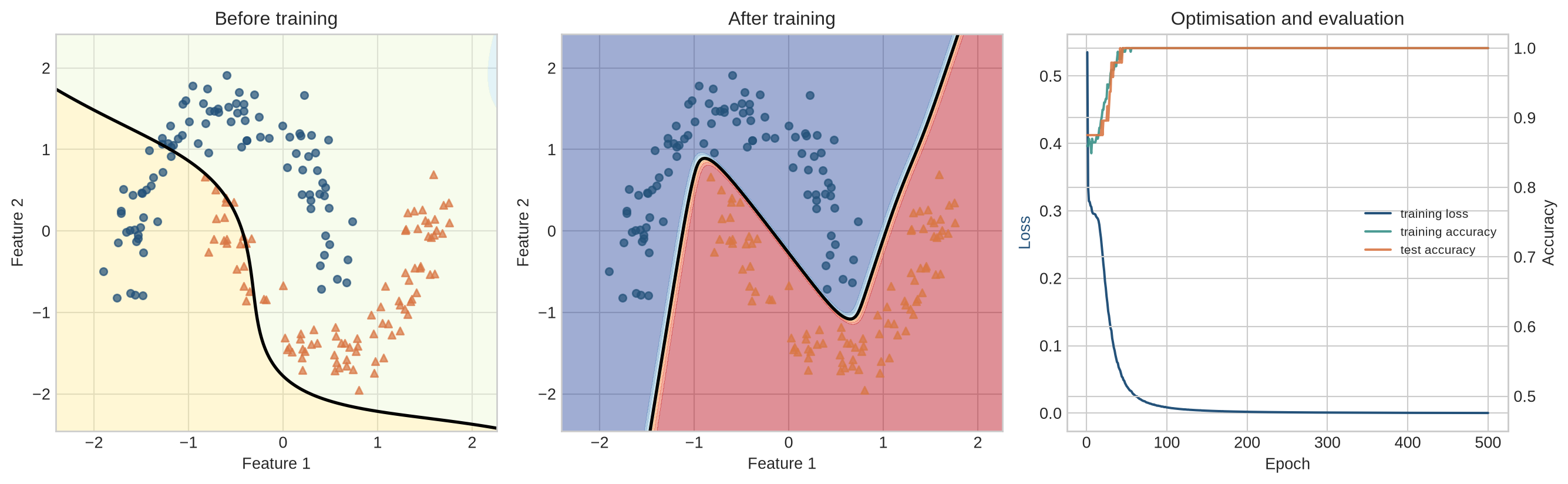
#| fig-cap: "Training lowers the batch-averaged loss and changes an initially arbitrary boundary into one that follows the curved class pattern."
#| fig-alt: "Three panels show the untrained boundary, trained boundary, and curves for training loss plus training and test accuracy across 500 epochs."
grid_x,grid_y=np.meshgrid(np.linspace(X_train_np[:,0].min()-0.5,X_train_np[:,0].max()+0.5,220),
                          np.linspace(X_train_np[:,1].min()-0.5,X_train_np[:,1].max()+0.5,220))
grid=torch.tensor(np.column_stack([grid_x.ravel(),grid_y.ravel()]),dtype=torch.float32)
trained_state={name:value.detach().clone() for name,value in model.state_dict().items()}
with torch.no_grad(): trained_surface=torch.sigmoid(model(grid)).numpy().reshape(grid_x.shape)
model.load_state_dict(initial_state)
with torch.no_grad(): initial_surface=torch.sigmoid(model(grid)).numpy().reshape(grid_x.shape)
model.load_state_dict(trained_state)

fig,axes=plt.subplots(1,3,figsize=(14,4.4))
for ax,surface,title in zip(axes[:2],[initial_surface,trained_surface],["Before training","After training"]):
    ax.contourf(grid_x,grid_y,surface,levels=np.linspace(0,1,11),cmap="RdYlBu_r",alpha=0.48)
    ax.contour(grid_x,grid_y,surface,levels=[0.5],colors="black",linewidths=2)
    for class_value,colour,marker in [(0,blue,"o"),(1,orange,"^")]:
        mask=y_train_np==class_value
        ax.scatter(X_train_np[mask,0],X_train_np[mask,1],c=colour,marker=marker,s=22,alpha=0.72)
    ax.set_title(title); ax.set_xlabel("Feature 1"); ax.set_ylabel("Feature 2")
epoch_axis=np.arange(1,epochs+1)
axes[2].plot(epoch_axis,history["loss"],color=blue,label="training loss")
accuracy_axis=axes[2].twinx()
accuracy_axis.plot(epoch_axis,history["train_accuracy"],color=teal,label="training accuracy",alpha=0.9)
accuracy_axis.plot(epoch_axis,history["test_accuracy"],color=orange,label="test accuracy",alpha=0.9)
axes[2].set_xlabel("Epoch"); axes[2].set_ylabel("Loss",color=blue)
accuracy_axis.set_ylabel("Accuracy"); accuracy_axis.set_ylim(0.45,1.02)
axes[2].set_title("Optimisation and evaluation")
lines1,labels1=axes[2].get_legend_handles_labels(); lines2,labels2=accuracy_axis.get_legend_handles_labels()
axes[2].legend(lines1+lines2,labels1+labels2,loc="center right",fontsize=8)
plt.tight_layout(); plt.show()
```
The initial boundary is determined by random initialisation. The trained boundary follows the curved pattern because the hidden activations allow the effective slope to change across input regions. The loss records the training objective; the accuracy curves apply a threshold and discard information about confidence. They answer different questions and need not move together at every epoch.
### A checkpoint must match the intended recovery task
```{python}
checkpoint={"epoch":epochs,"model_state":model.state_dict(),
            "optimiser_state":optimiser.state_dict(),"train_mean":train_mean,
            "train_std":train_std,"history":history,"torch_rng_state":torch.get_rng_state()}
print(checkpoint.keys())
```
Weights alone are enough for inference if the architecture and input transformation are known. Resuming training also requires optimiser state, the completed epoch or step, and enough configuration to recreate data processing and scheduling. Random-number state may be needed when exact continuation is required. A checkpoint is part of the training procedure, not merely a copy of the weights.
## Level 4 - Research & Systems
### The example loop implements stochastic optimisation
Mini-batch training estimates the full-data gradient using subsets of observations. The updates are cheaper than full-batch updates and contain sampling variation. Their behaviour depends on batch construction, learning rate, momentum or adaptive state, and observation order. Large-scale analyses therefore treat batch size and update rules jointly [@bottou2018].
The code uses Adam, which maintains estimates based on first and second moments of recent gradients [@kingma2014]. Those additional values increase optimiser memory and checkpoint size. Replacing Adam with plain stochastic gradient descent leaves the structure of the loop unchanged but changes the update calculation. Later chapters compare optimisers and schedules directly.
### Batch size exchanges memory and update frequency
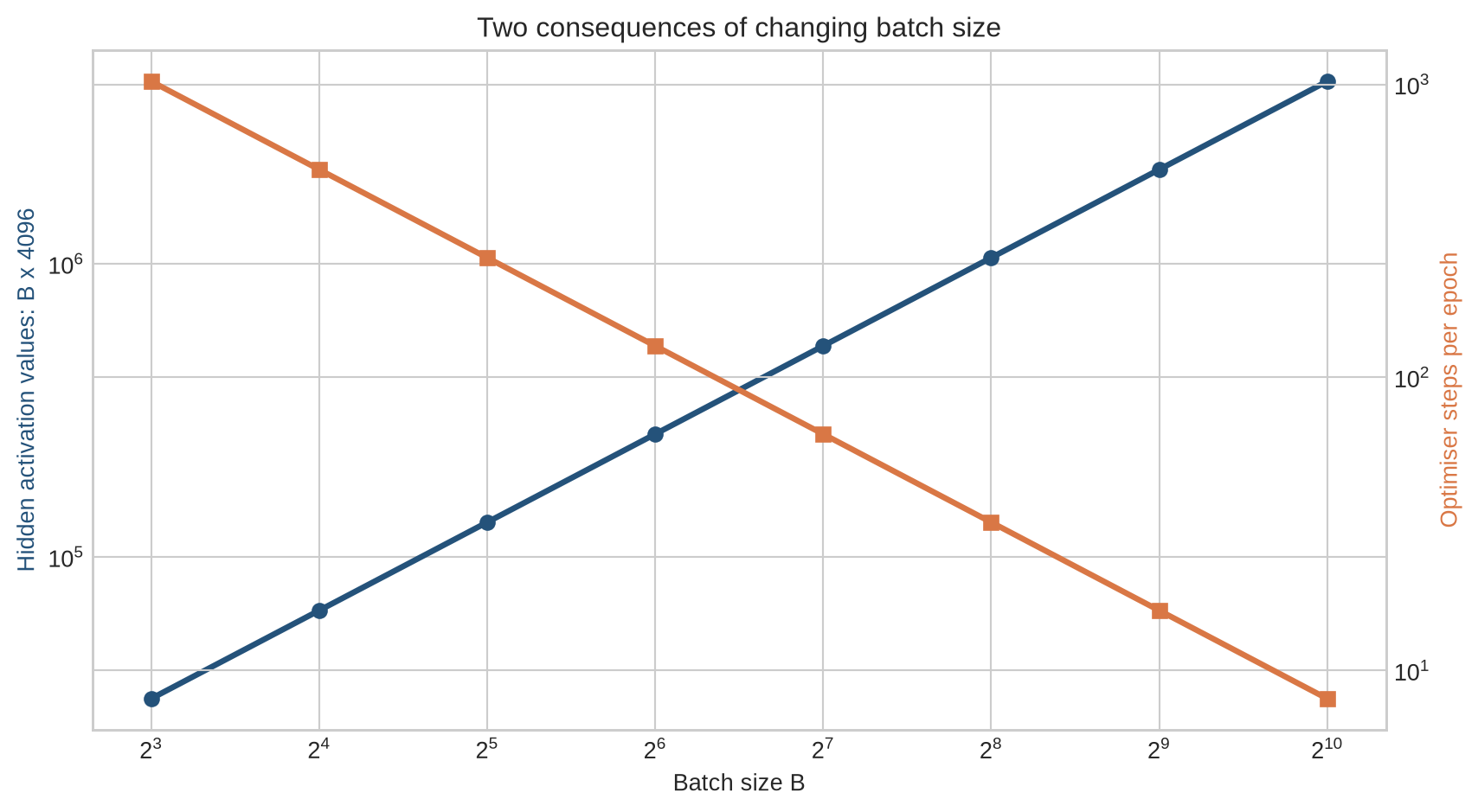
For $N$ observations, batch size $B$ produces approximately $\lceil N/B\rceil$ optimiser steps per epoch. Activation memory generally grows with $B$, while sampling variation in the batch gradient tends to decrease as batches include more observations. Neither relationship determines the best batch size by itself.
```{python}
#| label: fig-batch-tradeoffs
#| fig-cap: "For a fixed dataset, larger batches increase a simple activation-memory proxy and reduce the number of optimiser steps per epoch."
#| fig-alt: "A two-axis line chart shows activation values increasing with batch size while optimiser steps per epoch decrease for 8192 observations and hidden width 4096."
batch_sizes=np.array([8,16,32,64,128,256,512,1024]); dataset_size=8192; hidden_width=4096
activation_values=batch_sizes*hidden_width; steps_per_epoch=np.ceil(dataset_size/batch_sizes)
fig,ax1=plt.subplots(figsize=(9,5))
ax1.plot(batch_sizes,activation_values,marker="o",color=blue,linewidth=2.5)
ax1.set_xscale("log",base=2); ax1.set_yscale("log"); ax1.set_xlabel("Batch size B")
ax1.set_ylabel("Hidden activation values: B x 4096",color=blue)
ax2=ax1.twinx(); ax2.plot(batch_sizes,steps_per_epoch,marker="s",color=orange,linewidth=2.5)
ax2.set_yscale("log"); ax2.set_ylabel("Optimiser steps per epoch",color=orange)
ax1.set_title("Two consequences of changing batch size")
plt.tight_layout(); plt.show()
```
The memory line counts one hidden activation tensor and omits gradients, temporary buffers, and other layers, so it is not a memory forecast. The steps line assumes one update per batch. Gradient accumulation changes the effective batch size without requiring every observation to be resident at once, but it does not remove their computation.
### Framework automation does not remove experimental choices
PyTorch records operations dynamically and uses automatic differentiation to calculate gradients [@paszke2019]. The framework does not decide whether the split leaks information, whether the loss matches the objective, or whether a random result is stable. Those remain properties of the analysis and experimental design.
Reproducible reporting requires more than setting one seed. Code, data transformations, split definitions, software versions, hardware, hyperparameters, stopping criteria, and the number of runs can affect a reported result. @pineau2021 describe the NeurIPS reproducibility programme and its reporting checklist. Exact bitwise replication and replication of a substantive conclusion should be distinguished.
### Mixed precision changes representation, not the objective
Mixed-precision training stores or computes selected tensors in lower precision while retaining higher precision where needed for stability [@micikevicius2018]. This can reduce memory use and increase accelerator throughput. Small gradients may underflow, which motivates loss scaling. The mathematical objective is unchanged, but the numerical path used to estimate and apply its gradients differs.
The same distinction applies to fused optimisers and compiled training steps. They may combine operations, reduce kernel launches, or alter memory traffic while preserving the intended update within numerical tolerances. Validation should compare task outcomes and numerical behaviour in the target environment.
### Distributed data parallelism adds coordination
Data-parallel training gives different mini-batches to several workers. Each worker runs a forward and backward pass, after which gradients are communicated and combined before parameters are updated. PyTorch's distributed design overlaps parts of gradient communication with backpropagation [@li2020ddp]. The conceptual loop remains recognisable, but failures now include worker imbalance, communication stalls, inconsistent data sharding, and incomplete distributed checkpoints.
### A production training audit follows state across time
An auditable run should record:
- the dataset version, split logic, and fitted preprocessing state;
- architecture, initialisation, loss, optimiser, and schedule;
- batch construction, gradient accumulation, clipping, and numerical precision;
- training and evaluation modes, including stochastic layers;
- checkpoint contents and tested recovery behaviour;
- random seeds, software environment, hardware, and determinism settings;
- loss, validation metrics, gradient diagnostics, throughput, and failures;
- the rule used to select the final checkpoint.
A scalar final accuracy cannot reconstruct these decisions. The training loop is a stateful process, and its evidence consists of the configuration, data lineage, intermediate measurements, and resulting model together.
## Common misconceptions
- **The optimiser updates predictions directly.** It updates parameters; predictions are recalculated through the revised model.
- **Calling `backward()` updates the model.** It calculates and stores gradients. The optimiser step applies the update.
- **Gradients disappear automatically after an update.** PyTorch accumulates them until they are cleared or set to `None`.
- **Sigmoid must be applied before `BCEWithLogitsLoss`.** The loss expects logits and performs the stable combined calculation internally.
- **One epoch means one parameter update.** With mini-batches, an epoch contains several updates.
- **Evaluation mode disables gradients.** `model.eval()` changes layer behaviour; gradient tracking is disabled separately.
- **Training accuracy measures generalisation.** It measures performance on observations used for fitting.
- **A lower loss always changes accuracy.** Loss can improve without crossing a classification threshold.
- **Saving weights is a complete training checkpoint.** Resuming may also require optimiser, preprocessing, step, and random state.
- **Setting a seed guarantees identical results everywhere.** Software, hardware, operation choice, and parallel execution can differ.
- **A larger batch is always faster.** It may improve utilisation, exhaust memory, or reduce update frequency.
- **Distributed training eliminates the cost of larger models.** It adds communication and coordination.
## Exercises
1. Draw the dependency chain from input batch to parameter update.
2. Verify the three hidden pre-activations in the manual network.
3. Calculate its logit, probability, and binary cross-entropy loss.
4. Derive $\partial L/\partial s=p-y$.
5. Calculate `dW2`, `db2`, `dW1`, and `db1` for the worked observation.
6. Explain why the second row of `dW1` is zero.
7. Apply one learning-rate-$0.1$ update and recalculate the loss.
8. Calculate the parameter count of the $2\rightarrow16\rightarrow1$ model.
9. Rewrite the loop using full-batch gradient descent.
10. Remove `zero_grad()` for two batches and inspect the gradients.
11. Replace tanh with ReLU and compare at least five seeds.
12. Implement explicit sigmoid and binary cross-entropy with numerical safeguards.
13. Change the threshold to 0.3 and compare false positives and false negatives.
14. Add a validation split and distinguish it from the test set.
15. Save and reload the full checkpoint, then continue training.
16. Calculate steps per epoch for batch sizes 32, 128, and 512 when $N=8192$.
17. Explain which state is synchronised in data-parallel training.
18. Write a reproducibility record for the example.
## Summary
A training loop processes a batch, calculates logits and loss, backpropagates gradients, and updates parameters. The order is fixed by the computation graph. Clearing gradients is separate because PyTorch accumulates them. Evaluation removes the backward pass and update, changes the model to evaluation mode, and normally disables gradient tracking.
The classifier combines a $2\rightarrow16$ layer, tanh, and a $16\rightarrow1$ output layer. Training changes an initially arbitrary boundary into a curved boundary following the synthetic pattern. The loss and accuracy describe this generated dataset and run; they do not establish performance for another population.
At scale, the loop is modified by batching, gradient accumulation, mixed precision, compilation, checkpointing, and distributed communication. These changes preserve the dependency chain but alter state, numerical behaviour, memory use, and recovery requirements. Reproducible evidence must cover the training process rather than the final weights alone.
## Looking ahead
The example fits training and held-out observations generated by the same synthetic process. [Chapter 9](09-generalisation-overfitting.qmd) examines why fitting training data can diverge from performance on new data, how capacity and sampling variation contribute to overfitting, and what evidence is needed to assess generalisation.
## Further reading
Large-scale stochastic optimisation is reviewed by @bottou2018, while Adam is introduced by @kingma2014. PyTorch's execution and automatic-differentiation design are described by @paszke2019. Mixed-precision training is developed by @micikevicius2018, and data-parallel training is analysed by @li2020ddp. Reporting and experimental reproducibility are discussed by @pineau2021.