---
title: "Neural Network Layers"
subtitle: "From one output to structured representations"
---
## The problem
Chapter 5 turned the three prepared values for one household into one score. That is enough when a calculation is making the final prediction, but an intermediate part of a network often needs several values to carry forward. One value might respond to a pattern involving travel time and earlier contact; another might respond to a different combination of the same information. A later calculation can use all of them.
A neural-network layer produces those several values. It repeats the neuron calculation with different learned settings and places the results in a new vector. This chapter keeps the three household inputs from Chapter 5 so that the only new idea is the move from one output to several.
### The running calculation
The input remains the three-feature vector used in [Chapter 5](05-artificial-neuron.qmd):
$$
x=(2,4,1).
$$
Instead of producing one value, the layer will produce three. For now, it is enough to see that each output uses the same input vector but a different set of learned weights and its own bias. The exact numbers and the compact matrix notation appear after the layer's job is clear.
## Level 1 - Intuition
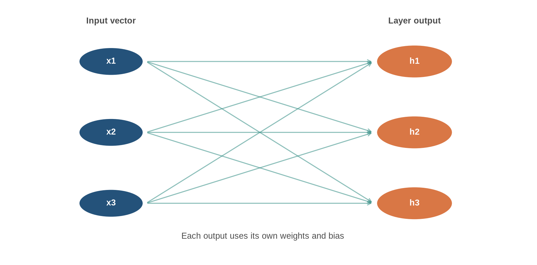
In the diagram, every output unit receives the same three input values, but it uses a different set of weights. Follow one arrow pattern to one orange circle: that is the Chapter 5 calculation with its own parameters. Then look at all three orange circles together: they are the values passed to the next calculation.
### A layer asks several questions of the same input
A neuron combines all available inputs into one output. A layer repeats that structure with different weights and biases. Every unit receives the same input vector, but each unit calculates a different weighted combination. The outputs are collected into a new vector.
```{python}
#| label: fig-layer-intuition
#| fig-cap: "A dense layer applies several different weighted combinations to the same input vector."
#| fig-alt: "Three input features connect to three output units. Every input connects to every output, and the three outputs form a new vector."
import numpy as np
import matplotlib.pyplot as plt
from matplotlib.patches import Circle, FancyArrowPatch

plt.style.use("seaborn-v0_8-whitegrid")
blue, teal, orange = "#24527a", "#3a9188", "#d97745"

fig, ax = plt.subplots(figsize=(9, 4.5))
input_y = np.array([0.78, 0.50, 0.22])
output_y = np.array([0.78, 0.50, 0.22])

for i, ypos in enumerate(input_y, start=1):
    ax.add_patch(Circle((0.18, ypos), 0.055, facecolor=blue, edgecolor="white", linewidth=1.2))
    ax.text(0.18, ypos, f"x{i}", ha="center", va="center", color="white", weight="bold")

for j, ypos in enumerate(output_y, start=1):
    ax.add_patch(Circle((0.70, ypos), 0.065, facecolor=orange, edgecolor="white", linewidth=1.2))
    ax.text(0.70, ypos, f"h{j}", ha="center", va="center", color="white", weight="bold")

for y_in in input_y:
    for y_out in output_y:
        ax.add_patch(FancyArrowPatch(
            (0.24, y_in),
            (0.63, y_out),
            arrowstyle="->",
            mutation_scale=10,
            linewidth=1.2,
            color=teal,
            alpha=0.58,
        ))

ax.text(0.18, 0.93, "Input vector", ha="center", color="#4a4a4a", weight="bold")
ax.text(0.70, 0.93, "Layer output", ha="center", color="#4a4a4a", weight="bold")
ax.text(0.44, 0.08, "Each output uses its own weights and bias", ha="center", color="#4a4a4a")
ax.set_xlim(0, 0.9)
ax.set_ylim(0, 1)
ax.axis("off")
plt.tight_layout()
plt.show()
```
The diagram is fully connected because each output uses all three inputs. The three orange circles do not vote on one decision. They form a three-value output, which becomes the input to the next layer.
::: {.concept-box .concept-core #concept-neural-layer data-term="Neural-network layer" data-domain="Foundations" data-symbols="W; b"}
**Neural-network layer.** Several neuron calculations applied to the same input. Each one has its own learned weights and bias; together their outputs form a new vector for the next calculation.
:::
### A layer changes the representation
The original coordinates describe information supplied to the model. A hidden layer produces new coordinates defined by its learned settings. One output may be high for one combination of the inputs and another for a different combination. These outputs are called a **representation** because they describe the same household in a form that later layers can use.
The individual coordinates should not automatically be assigned human-readable concepts. A layer is trained as part of a larger objective, and useful information can be distributed across many units. The relevant claim is computational: the layer has transformed one vector into another.
### Width and depth describe different choices
The **width** of a layer is its number of output units. A layer with 128 outputs is wider than one with 32. The **depth** of a network counts successive parameterised layers along the computation path. Adding units changes how much a layer can represent at one stage. Adding layers changes how many transformations are composed.
The distinction is structural, not evaluative. A wider or deeper network is not automatically better. It has a different parameter count, computational cost, and set of functions it can represent. Whether that additional capacity improves performance depends on the data, training procedure, and evaluation setting.
### Input, hidden, and output layers
The phrase **input layer** usually refers to the values supplied to the network rather than a learned calculation. A **hidden layer** produces an internal representation that is passed onwards. An **output layer** maps the final hidden representation to the form required by the task, such as one regression score or a set of class logits.
These names describe position in the network. The matrix operation can be the same in a hidden layer and an output layer even though their outputs have different interpretations.
The layer has increased the number of values carried forward without changing the basic arithmetic. The next level works through three such calculations, one output at a time, before introducing the matrix that stores them together.
## Level 2 - Mechanics
The layer diagram can now be read as three concrete calculations. Each one combines the same input values, but it has a different set of weights and a different bias.
### Three calculations, one input
For the running example, the three outputs are calculated separately:
| Unit | Weighted sum | Bias | Pre-activation | ReLU output |
|---:|---|---:|---:|---:|
| 1 | $0.5(2)-1(4)+2(1)=-1$ | $3$ | $2$ | $2$ |
| 2 | $-0.25(2)+0.5(4)+1(1)=2.5$ | $-1$ | $1.5$ | $1.5$ |
| 3 | $1(2)+0.25(4)-0.5(1)=2.5$ | $-4$ | $-1.5$ | $0$ |
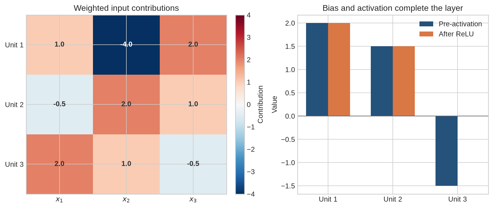
The third pre-activation is negative, so ReLU replaces it with zero. The layer output is therefore $(2,1.5,0)$.
```{python}
#| label: fig-layer-mechanics
#| fig-cap: "Rows of the weight matrix define output units; row sums and biases produce the pre-activation vector."
#| fig-alt: "A heatmap shows the nine weighted input contributions for three units. A bar chart shows the three pre-activations and their ReLU outputs."
x_mech = np.array([2.0, 4.0, 1.0])
W_mech = np.array([
    [0.5, -1.0, 2.0],
    [-0.25, 0.5, 1.0],
    [1.0, 0.25, -0.5],
])
b_mech = np.array([3.0, -1.0, -4.0])
contribution_matrix = W_mech * x_mech[np.newaxis, :]
z_mech = contribution_matrix.sum(axis=1) + b_mech
h_mech = np.maximum(0, z_mech)

fig, axes = plt.subplots(1, 2, figsize=(10, 4.3), gridspec_kw={"width_ratios": [1.15, 1]})
image = axes[0].imshow(contribution_matrix, cmap="RdBu_r", vmin=-4, vmax=4, aspect="auto")
for row in range(contribution_matrix.shape[0]):
    for col in range(contribution_matrix.shape[1]):
        value = contribution_matrix[row, col]
        axes[0].text(col, row, f"{value:.1f}", ha="center", va="center",
                     color="white" if abs(value) > 2.2 else "#303030", weight="bold")
axes[0].set_xticks(range(3), [r"$x_1$", r"$x_2$", r"$x_3$"])
axes[0].set_yticks(range(3), ["Unit 1", "Unit 2", "Unit 3"])
axes[0].set_title("Weighted input contributions")
fig.colorbar(image, ax=axes[0], fraction=0.046, pad=0.04, label="Contribution")

positions = np.arange(3)
bar_width = 0.34
axes[1].bar(positions - bar_width / 2, z_mech, bar_width, color=blue, label="Pre-activation")
axes[1].bar(positions + bar_width / 2, h_mech, bar_width, color=orange, label="After ReLU")
axes[1].axhline(0, color="#666666", linewidth=0.9)
axes[1].set_xticks(positions, ["Unit 1", "Unit 2", "Unit 3"])
axes[1].set_ylabel("Value")
axes[1].set_title("Bias and activation complete the layer")
axes[1].legend(frameon=False)

plt.tight_layout()
plt.show()
```
The heatmap preserves information hidden by the final sum. The first row contains a contribution of $-4$ from the second input, which is offset by the first and third contributions and the bias. The bar chart then separates the affine result from the activation. This distinction matters because the weight matrix and bias define the affine layer, while ReLU is a separate operation.
### Rows are units and columns are inputs
The orientation of the weight matrix is a common source of confusion. In this book, and in PyTorch's linear layer:
- each **row** contains the weights for one output unit;
- each **column** corresponds to one input feature;
- the number of rows is the output width; and
- the number of columns is the input width.
A $3\times3$ matrix is ambiguous by inspection because the input and output widths happen to match. For a layer with three inputs and five outputs, the weight matrix has five rows and three columns. Writing the dimensions before calculating prevents many shape errors.
### Layers compose by matching dimensions
Suppose the first layer maps three inputs to four hidden values. A second layer can consume those values only if its input width is four. If it produces two outputs, the shape sequence for one observation is:
$$
(3)\rightarrow(4)\rightarrow(2).
$$
For a batch of size $B$, the same sequence is:
$$
(B,3)\rightarrow(B,4)\rightarrow(B,2).
$$
The adjacent dimensions must match. A network architecture is therefore partly a contract between layers: the output width of one layer becomes the input width of the next.
### Training changes the matrix, not the layer rule
During the forward pass, the layer uses its current $W$ and $b$. Backpropagation calculates a gradient for every matrix and bias entry. The optimiser changes those entries, and the next forward pass uses the updated values. The rule $Z=XW^\top+b$ remains fixed; training changes the parameters inside that rule.
Once the rows, columns, and bias vector are visible, matrix notation becomes a bookkeeping device rather than an additional abstraction. The formalisation below tracks the same calculation for one input and then for a batch.
## Level 3 - Mathematics & Code
The mechanics can now be expressed with dimensions that remain valid when the input width, output width, and batch size differ. The code will implement the same calculation three ways and verify that the results agree.
### One observation
Let:
- $x\in\mathbb{R}^{d_{\mathrm{in}}}$ be one input vector;
- $W\in\mathbb{R}^{d_{\mathrm{out}}\times d_{\mathrm{in}}}$ be the weight matrix;
- $b\in\mathbb{R}^{d_{\mathrm{out}}}$ be the bias vector;
- $z\in\mathbb{R}^{d_{\mathrm{out}}}$ be the pre-activation; and
- $h\in\mathbb{R}^{d_{\mathrm{out}}}$ be the activated output.
The layer computes:
$$
z=Wx+b,
\qquad
h=g(z).
$$
The $j$th output is:
$$
z_j=\sum_{k=1}^{d_{\mathrm{in}}}W_{jk}x_k+b_j.
$$
The index $j$ selects one row of $W$, so it selects one output unit. The index $k$ runs across the inputs. The formula is the neuron equation from Chapter 5 repeated for every row.
### A batch
Let $X\in\mathbb{R}^{B\times d_{\mathrm{in}}}$ store $B$ observations as rows. PyTorch stores the weight matrix in output-by-input orientation, so the batch calculation is:
$$
Z=XW^\top+b,
$$
with:
$$
Z\in\mathbb{R}^{B\times d_{\mathrm{out}}}.
$$
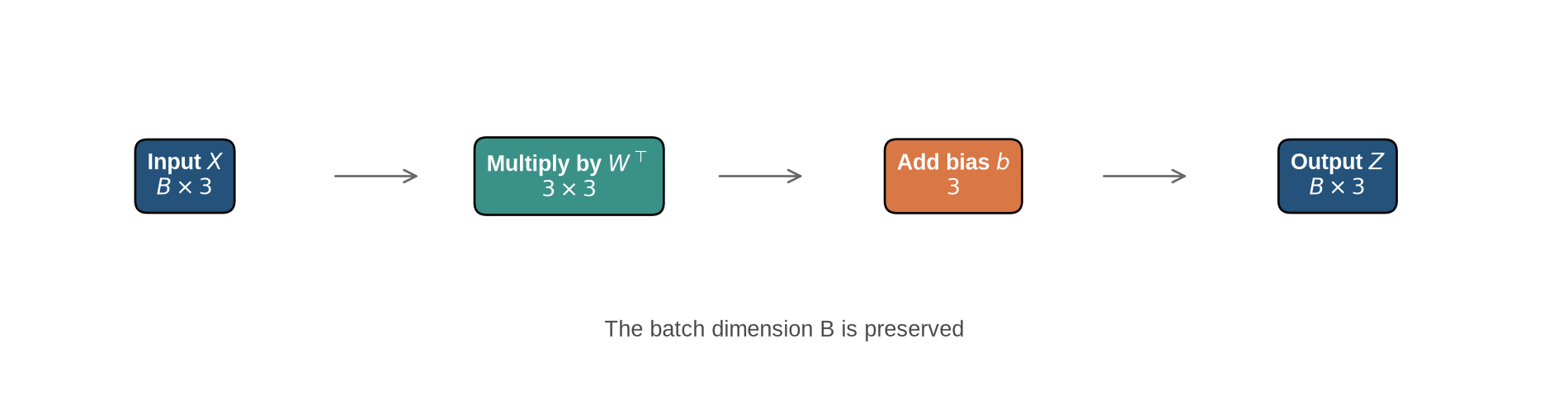
The bias vector is **broadcast** across the batch: the same $b_j$ is added to output $j$ for every observation. Broadcasting does not create separate learned biases for each observation.
| Object | Shape | Meaning |
|---|---|---|
| $X$ | $B\times d_{\mathrm{in}}$ | batch of input vectors |
| $W$ | $d_{\mathrm{out}}\times d_{\mathrm{in}}$ | one row per output unit |
| $b$ | $d_{\mathrm{out}}$ | one bias per output unit |
| $Z$ | $B\times d_{\mathrm{out}}$ | batch of pre-activation vectors |
The shape calculation makes two things visible. The layer changes the final dimension from input width to output width, and it does not mix observations within the batch. Every row uses the same $W$ and $b$.
```{python}
#| label: fig-batch-layer
#| fig-cap: "A batch changes the number of observations, while the layer determines the output width."
#| fig-alt: "A horizontal shape diagram shows an input batch of B by 3 multiplied by a transposed 3 by 3 weight matrix, followed by a bias, producing an output batch of B by 3."
fig, ax = plt.subplots(figsize=(10, 2.6))
blocks = [
    (0.11, r"Input $X$" + "\n" + r"$B \times 3$", blue),
    (0.36, r"Multiply by $W^\top$" + "\n" + r"$3 \times 3$", teal),
    (0.61, r"Add bias $b$" + "\n" + r"$3$", orange),
    (0.86, r"Output $Z$" + "\n" + r"$B \times 3$", blue),
]
for xpos, label, colour in blocks:
    ax.text(xpos, 0.56, label, ha="center", va="center", color="white", weight="bold",
            bbox={"boxstyle": "round,pad=0.55", "facecolor": colour})
for left, right in zip(blocks[:-1], blocks[1:]):
    ax.add_patch(FancyArrowPatch(
        (left[0] + 0.095, 0.56),
        (right[0] - 0.095, 0.56),
        arrowstyle="->",
        mutation_scale=14,
        color="#666666",
    ))
ax.text(0.5, 0.12, "The batch dimension B is preserved", ha="center", color="#4a4a4a")
ax.set_xlim(0, 1)
ax.set_ylim(0, 1)
ax.axis("off")
plt.tight_layout()
plt.show()
```
The same parameter values are reused for every row. This is why a trained layer can process a new household without acquiring a new set of weights.
### NumPy calculation
The following code calculates the running example without a neural-network library. Its purpose is to expose the matrix multiplication, bias addition, and activation separately.
```{python}
import numpy as np

x = np.array([2.0, 4.0, 1.0])
W = np.array([
    [0.5, -1.0, 2.0],
    [-0.25, 0.5, 1.0],
    [1.0, 0.25, -0.5],
])
b = np.array([3.0, -1.0, -4.0])

z_numpy = W @ x + b
h_numpy = np.maximum(0, z_numpy)

print("pre-activation:", z_numpy)
print("after ReLU:    ", h_numpy)
```
The matrix product returns $(2,1.5,-1.5)$. ReLU changes only the negative component, producing $(2,1.5,0)$. The code uses one matrix multiplication, but it is numerically identical to the three row-by-row calculations in Level 2.
### The same layer in PyTorch
PyTorch's `nn.Linear` stores $W$ with shape `(out_features, in_features)`. The activation remains a separate operation.
```{python}
import torch
import torch.nn as nn

torch_layer = nn.Linear(in_features=3, out_features=3)
with torch.no_grad():
    torch_layer.weight.copy_(torch.tensor(W, dtype=torch.float32))
    torch_layer.bias.copy_(torch.tensor(b, dtype=torch.float32))

x_torch = torch.tensor(x, dtype=torch.float32)
z_torch = torch_layer(x_torch)
h_torch = torch.relu(z_torch)

print("weight shape:  ", tuple(torch_layer.weight.shape))
print("bias shape:    ", tuple(torch_layer.bias.shape))
print("pre-activation:", z_torch.detach().numpy())
print("after ReLU:    ", h_torch.detach().numpy())
print("matches NumPy: ", np.allclose(h_numpy, h_torch.detach().numpy()))
```
The final line verifies that the NumPy and PyTorch outputs agree. This check is useful when translating an equation into a framework: matching values are stronger evidence than matching tensor shapes alone.
### Composing two layers
A two-layer forward computation can be written:
$$
h=g(W_1x+b_1),
$$
$$
s=W_2h+b_2.
$$
The first layer produces a hidden representation $h$. The second produces an output score $s$. For the running example, use:
$$
W_2=
\begin{bmatrix}
0.6 & -0.4 & 1.2
\end{bmatrix},
\qquad b_2=-0.2.
$$
Then:
$$
s=0.6(2)-0.4(1.5)+1.2(0)-0.2=0.4.
$$
```{python}
second_layer = nn.Linear(3, 1)
with torch.no_grad():
    second_layer.weight.copy_(torch.tensor([[0.6, -0.4, 1.2]]))
    second_layer.bias.copy_(torch.tensor([-0.2]))

network = nn.Sequential(torch_layer, nn.ReLU(), second_layer)
score = network(x_torch)
print(f"network score: {score.item():.1f}")
```
The score is $0.4$, matching the manual calculation. It is not yet a probability. An output interpretation requires an appropriate final transformation and loss, which depend on the task.
### Parameter counts
A dense layer has:
$$
d_{\mathrm{out}}d_{\mathrm{in}}
$$
weights and:
$$
d_{\mathrm{out}}
$$
biases. Its total parameter count is:
$$
d_{\mathrm{out}}d_{\mathrm{in}}+d_{\mathrm{out}}
=d_{\mathrm{out}}(d_{\mathrm{in}}+1).
$$
The first $3\rightarrow3$ layer has $3(3+1)=12$ parameters. The $3\rightarrow1$ output layer has $1(3+1)=4$. The two-layer network therefore has 16 parameters.
```{python}
parameter_table = []
total_parameters = 0
for name, parameter in network.named_parameters():
    count = parameter.numel()
    total_parameters += count
    parameter_table.append((name, tuple(parameter.shape), count))

for name, shape, count in parameter_table:
    print(f"{name:10s} shape={str(shape):8s} parameters={count}")
print("total parameters:", total_parameters)
```
The framework count agrees with the formula. Parameter counting should be done layer by layer because biases, embeddings, normalisation parameters, and tied weights can make a network total less obvious than a single dense-layer calculation.
### Gradient shapes
Let $G=\partial L/\partial Z$ contain the gradient arriving from the next operation, with shape $B\times d_{\mathrm{out}}$. For $Z=XW^\top+b$, the layer gradients are:
$$
\frac{\partial L}{\partial W}=G^\top X,
$$
$$
\frac{\partial L}{\partial b}=\sum_{i=1}^{B}G_{i,:}.
$$
The matrix product $G^\top X$ has shape $d_{\mathrm{out}}\times d_{\mathrm{in}}$, exactly matching $W$. The bias gradient sums over observations because the same bias was broadcast to every row during the forward pass.
```{python}
x_batch = torch.tensor([
    [2.0, 4.0, 1.0],
    [1.0, 0.0, 2.0],
], dtype=torch.float32)

network.zero_grad()
batch_scores = network(x_batch)
loss = (batch_scores ** 2).mean()
loss.backward()

for name, parameter in network.named_parameters():
    print(f"{name:10s} parameter={tuple(parameter.shape)} gradient={tuple(parameter.grad.shape)}")
```
Every gradient has the same shape as its parameter. Backpropagation does not produce one generic learning signal for a layer; it produces one derivative for every stored weight and bias.
## Level 4 - Research & Systems
The small layer fits comfortably in a table. Large models use the same algebra with dimensions that change memory use, arithmetic cost, and communication requirements. The relevant systems object is no longer an individual neuron but a matrix multiplication.
### Dense layers are matrix-multiplication kernels
For a batch matrix $X$ and weight matrix $W$, computing $XW^\top$ requires approximately:
$$
2B\,d_{\mathrm{in}}d_{\mathrm{out}}
$$
floating-point operations when a multiply and an addition are counted separately. The layer stores $d_{\mathrm{in}}d_{\mathrm{out}}$ weights and produces $B\,d_{\mathrm{out}}$ output activations.
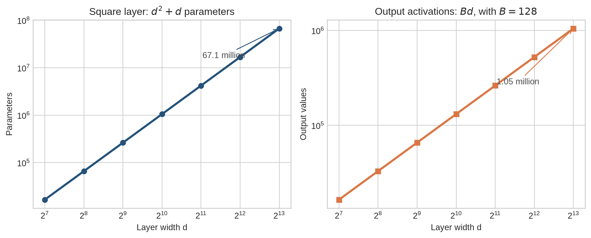
These quantities scale differently. For a square layer with width $d$, parameter count grows as $d^2$, while output activations for a fixed batch grow as $Bd$. Doubling width therefore approximately quadruples the weights but only doubles the output activation count.
```{python}
#| label: fig-layer-scaling
#| fig-cap: "For a square dense layer, parameter count grows quadratically with width while output activations grow linearly for a fixed batch."
#| fig-alt: "Two log-scale plots show square-layer parameters increasing faster than output activations as width rises from 128 to 8192."
widths = np.array([128, 256, 512, 1024, 2048, 4096, 8192])
batch_size = 128
square_parameters = widths ** 2 + widths
output_activations = batch_size * widths

fig, axes = plt.subplots(1, 2, figsize=(10, 4.1))
axes[0].plot(widths, square_parameters, marker="o", color=blue, linewidth=2.5)
axes[0].set_xscale("log", base=2)
axes[0].set_yscale("log")
axes[0].set(
    xlabel="Layer width d",
    ylabel="Parameters",
    title=r"Square layer: $d^2+d$ parameters",
)
axes[0].annotate(
    f"{square_parameters[-1] / 1e6:.1f} million",
    xy=(widths[-1], square_parameters[-1]),
    xytext=(2100, 1.6e7),
    arrowprops={"arrowstyle": "->", "color": blue},
    color="#4a4a4a",
)

axes[1].plot(widths, output_activations, marker="s", color=orange, linewidth=2.5)
axes[1].set_xscale("log", base=2)
axes[1].set_yscale("log")
axes[1].set(
    xlabel="Layer width d",
    ylabel="Output values",
    title=rf"Output activations: $B d$, with $B={batch_size}$",
)
axes[1].annotate(
    f"{output_activations[-1] / 1e6:.2f} million",
    xy=(widths[-1], output_activations[-1]),
    xytext=(2100, 2.7e5),
    arrowprops={"arrowstyle": "->", "color": orange},
    color="#4a4a4a",
)

plt.tight_layout()
plt.show()
```
At width 8,192, one square layer contains about 67 million parameters before optimiser state or gradients are counted. The plotted activation count covers only the layer output for a batch of 128, not every intermediate value retained for backpropagation. Parameter memory and activation memory must therefore be estimated separately.
### Layer shape determines memory traffic
A matrix multiplication needs the input activations and weights to be available to the accelerator, and it writes an output tensor. If a matrix is reused across many observations or token positions, the arithmetic performed per weight load can be high. Small or irregular operations may spend proportionally more time moving data than multiplying it.
This is why implementations combine compatible operations when possible. Bias addition and activation can be fused with, or scheduled close to, the matrix multiplication so that intermediate values do not make unnecessary trips through device memory. The mathematical layer is unchanged, but the execution plan affects latency and throughput.
### When one device cannot hold the matrix
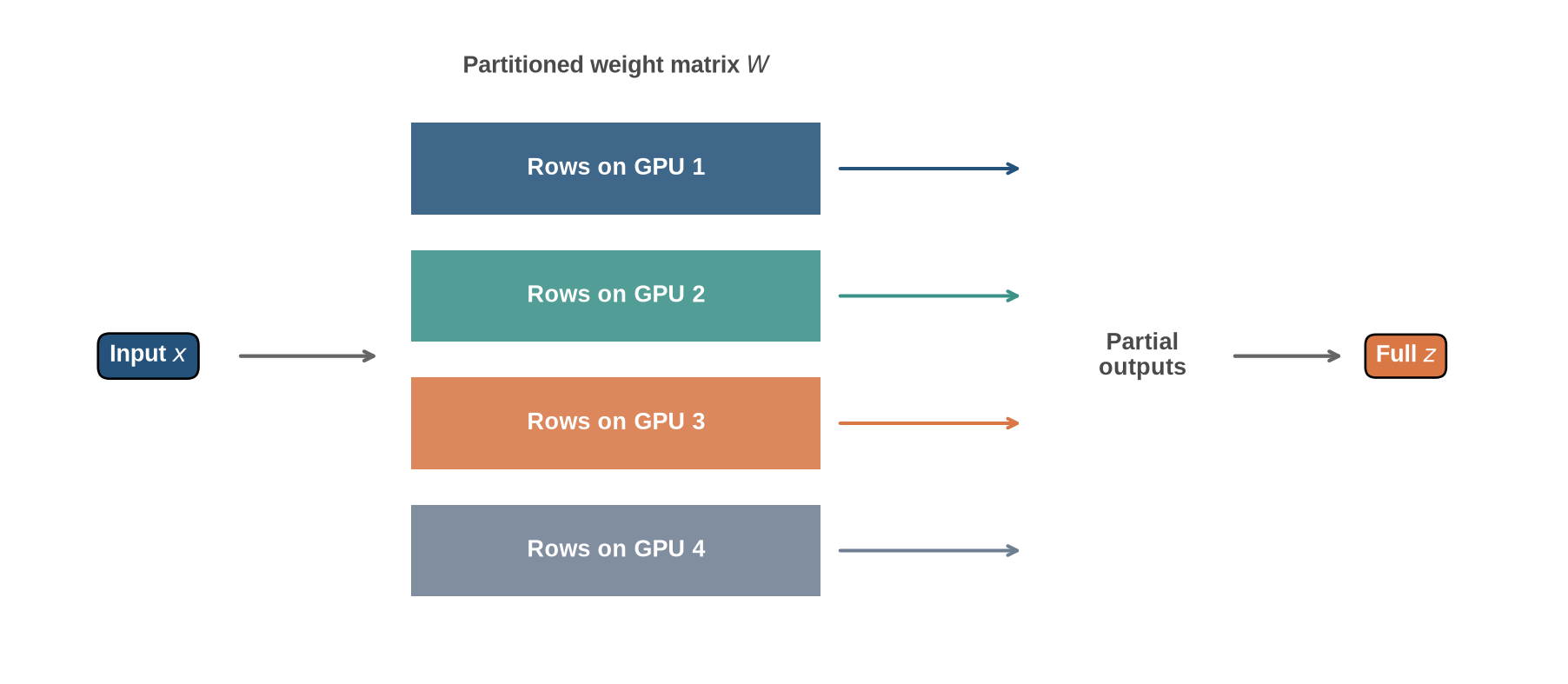
If a weight matrix is too large for one accelerator, it can be partitioned. **Tensor parallelism** splits the matrix operation itself across devices. One approach assigns different groups of output rows to different accelerators. Each device computes part of the output vector, and the parts are then concatenated or combined.
```{python}
#| label: fig-tensor-parallel-layer
#| fig-cap: "Tensor parallelism can divide the rows of a large weight matrix across accelerators."
#| fig-alt: "A weight matrix is divided into four horizontal blocks labelled GPU 1 to GPU 4. Each block produces part of the output, and the parts are combined into one vector."
from matplotlib.patches import Rectangle

fig, ax = plt.subplots(figsize=(9.5, 4.2))
gpu_colours = [blue, teal, orange, "#6f7f93"]
block_y = [0.72, 0.54, 0.36, 0.18]

ax.text(0.09, 0.52, r"Input $x$", ha="center", va="center", color="white", weight="bold",
        bbox={"boxstyle": "round,pad=0.5", "facecolor": blue})
ax.annotate("", xy=(0.25, 0.52), xytext=(0.15, 0.52),
            arrowprops={"arrowstyle": "->", "color": "#666666", "lw": 1.6})

for idx, (ypos, colour) in enumerate(zip(block_y, gpu_colours), start=1):
    ax.add_patch(Rectangle((0.27, ypos), 0.28, 0.13, facecolor=colour, alpha=0.88))
    ax.text(0.41, ypos + 0.065, f"Rows on GPU {idx}", ha="center", va="center",
            color="white", weight="bold")
    ax.annotate("", xy=(0.69, ypos + 0.065), xytext=(0.56, ypos + 0.065),
                arrowprops={"arrowstyle": "->", "color": colour, "lw": 1.5})

ax.text(0.77, 0.52, "Partial\noutputs", ha="center", va="center", color="#4a4a4a", weight="bold")
ax.annotate("", xy=(0.91, 0.52), xytext=(0.83, 0.52),
            arrowprops={"arrowstyle": "->", "color": "#666666", "lw": 1.6})
ax.text(0.95, 0.52, r"Full $z$", ha="center", va="center", color="white", weight="bold",
        bbox={"boxstyle": "round,pad=0.45", "facecolor": orange})
ax.text(0.41, 0.92, r"Partitioned weight matrix $W$", ha="center", color="#4a4a4a", weight="bold")
ax.set_xlim(0, 1.05)
ax.set_ylim(0.08, 1)
ax.axis("off")
plt.tight_layout()
plt.show()
```
The figure shows a row-wise partition for explanation; production systems also use column-wise partitions and combine them across successive operations. Megatron-LM demonstrated that intra-layer model parallelism can distribute large Transformer matrix multiplications with a small number of communication operations [@shoeybi2019]. The benefit depends on whether reduced per-device memory and computation compensate for communication between devices.
### Depth, width, and expressivity
Successive layers can create functions that would require many more units in a shallower architecture, but such statements depend on the activation, function class, and approximation criterion. Research on neural-network expressivity therefore studies specific architectural families rather than treating depth as a universal measure of intelligence. Raghu and colleagues analyse how trajectory-based measures of functional complexity change with depth [@raghu2017expressive].
The practical choice of depth and width also involves optimisation and generalisation. A network can have enough representational capacity and still train poorly, overfit, or fail under distribution shift. Parameter count describes architecture; it does not establish that the parameters can be estimated reliably from the available data.
### Not every layer is dense
A dense layer gives every output its own weight for every input. Other layer types impose structure:
- convolutional layers reuse local filters across spatial positions;
- attention layers calculate input-dependent weighted combinations across sequence positions;
- embedding layers retrieve learned rows from a table; and
- mixture-of-experts layers route an input through a subset of available parameter blocks.
These operations still transform tensors and expose parameters to backpropagation, but their connectivity and parameter sharing differ from a dense matrix. Later chapters will derive them separately. Treating every layer as `nn.Linear` would hide the architectural assumptions that make those models useful.
### What should be measured in a real system
For a layer or block, a systems audit should record:
- input and output shapes, including batch and sequence dimensions;
- parameter count and numerical precision;
- activation sizes needed during training;
- forward and backward execution time;
- communication introduced by parallelism; and
- whether the measured operation is limited by arithmetic, memory movement, or synchronisation.
The matrix dimensions provide a first estimate, but measured performance depends on the accelerator, kernel library, surrounding operations, and degree of parallelism. A parameter count alone cannot predict training time or inference latency.
## Common misconceptions
- **A layer is one neuron with more inputs.** A dense layer contains several output units and returns a vector.
- **Each hidden unit must correspond to one interpretable concept.** Useful information can be distributed across many coordinates.
- **The batch size changes the number of learned weights.** The same weights are reused for every observation in the batch.
- **Rows of a PyTorch weight matrix correspond to inputs.** Rows correspond to outputs; columns correspond to inputs.
- **The bias has one value per input.** A dense layer normally has one bias per output unit.
- **A wider layer always improves the model.** Width increases capacity and cost, but performance depends on data and training.
- **Stacking affine layers is enough to obtain a nonlinear network.** Without nonlinear operations between them, the composition remains affine.
- **Parameter count determines memory use.** Training also stores gradients, optimiser state, and activations.
- **A matrix split across GPUs eliminates communication.** Partial results must still be combined or passed between partitions.
- **All neural-network layers are dense.** Convolution, attention, embeddings, and expert routing use different connectivity.
## Exercises
1. A layer receives four inputs and produces six outputs. Write the shapes of $W$, $b$, and $z$ for one observation.
2. Write the corresponding shapes for a batch of 32 observations.
3. Calculate the parameter count of the $4\rightarrow6$ layer, including biases.
4. Use the running-example matrix to calculate the second pre-activation by hand.
5. Explain why the third output becomes zero after ReLU.
6. Describe the difference between a layer's width and a network's depth.
7. A network has shape sequence $10\rightarrow20\rightarrow5\rightarrow1$. Calculate the parameter count of each dense layer and the total.
8. Implement the running example using NumPy without a loop over output units.
9. Reproduce the same calculation with `nn.Linear` and verify numerical agreement.
10. Explain why the bias gradient sums across observations in a batch.
11. For $B=64$, $d_{\mathrm{in}}=1024$, and $d_{\mathrm{out}}=4096$, calculate the number of output activation values and the layer's parameter count.
12. Explain why doubling the width of a square dense layer approximately quadruples its parameter count.
13. Give one reason tensor parallelism can make a layer feasible and one reason it may reduce efficiency.
14. Compare a dense layer with one structured layer type named in Level 4. Which weights are shared or omitted?
15. A model receives a tensor of shape $(32,10)$ but a layer was constructed with `in_features=12`. Identify the incompatible dimensions and state one legitimate repair.
16. For a $512\rightarrow2048\rightarrow512$ block, calculate the parameter count of both layers including biases. Explain why the intermediate width, rather than the input or output width alone, determines most of the parameter cost.
## Summary
A dense layer applies several neuron-equivalent calculations at once. For one observation it computes $z=Wx+b$; for a batch it computes $Z=XW^\top+b$ when weights are stored in output-by-input orientation. Rows of $W$ define output units, columns correspond to inputs, and the bias has one entry per output.
Layer composition requires adjacent dimensions to match. Parameter counts grow with input and output width, while backpropagation produces gradients with the same shapes as the stored parameters. At scale, dense layers are matrix-multiplication kernels whose feasibility depends on parameter memory, activation memory, numerical precision, and communication. Tensor parallelism can split a matrix across accelerators, but it exchanges local memory constraints for coordination costs.
## Looking ahead
Layers can be composed without producing a genuinely nonlinear model. [Chapter 7](07-activation-functions.qmd) examines the activation functions placed between layers, how they change representation and gradient flow, and why different architectures use different nonlinearities.
## Further reading
The relationship between multilayer networks and backpropagation is developed by @rumelhart1986. @raghu2017expressive examine how architectural depth affects measures of expressivity. Dense feed-forward layers within Transformers are described by @vaswani2017. Intra-layer tensor parallelism for large language models is presented by @shoeybi2019.