---
title: "Sequence Modelling Before Transformers"
subtitle: "Order, recurrent state, and the fixed-memory bottleneck"
---
## The problem
Chapter 17 gave each discrete item a learned vector, and Chapter 16 showed how such vectors sit along a sequence axis. Nothing so far represents order. A reduction that sums or averages the position vectors returns the same summary for `red then blue` and for `blue then red`, yet many tasks depend on which item came first and on which earlier information is still available when a later item is processed.
A recurrent neural network addresses order by carrying a state from one position to the next: the representation at each position is computed from the current input together with whatever the state retains of earlier positions. That single mechanism raises the questions this chapter answers. What can a fixed-width state hold, and how is it updated? How do gradients reach early positions through a chain of repeated transitions? When may a model use future positions, and when must it not? And what happens when an entire source sequence must pass through one final state before a decoder begins? These limitations explain later design choices: gates that regulate what is retained, bidirectional encoders for tasks that permit future context, and the attention mechanism that Chapter 19 introduces.
### A delayed-copy task makes retention visible
The running task is a constructed delayed-copy problem. The first position contains either $+1$ or $-1$; the remaining positions contain zeros; at the final position the model must return the first signal. The task is deliberately simple: success requires retaining one early value across a growing number of steps, so failures of state and gradient propagation become visible. Results from this task illustrate mechanics; they are not evidence about natural sequence data.
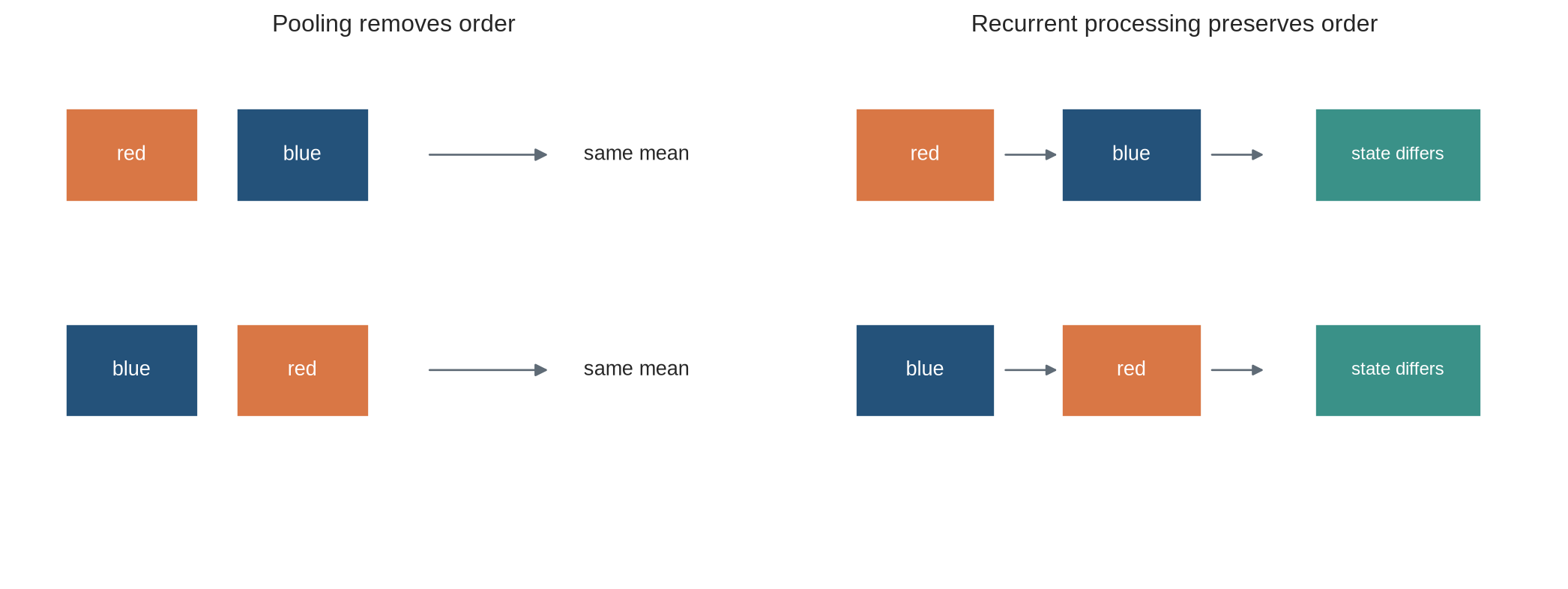
The first diagram contrasts two ways of handling the same pair of sequences. The left panel pools the position vectors and loses the order; the right panel applies a recurrent update, so the final state can differ between the two orders. Notice that the difference comes from the direction of information flow, not from different inputs.
```{python}
#| label: fig-order-sensitive
#| fig-cap: "Order-insensitive pooling gives the same summary to reversed sequences, while a recurrent update can produce different states."
#| fig-alt: "Two sequences containing red and blue in opposite orders have identical pooled vectors but follow different arrows through recurrent state boxes and end at different states."
import numpy as np
import matplotlib.pyplot as plt
from matplotlib.patches import Rectangle, FancyArrowPatch

plt.style.use("seaborn-v0_8-whitegrid")
blue, teal, orange, purple, grey = "#24527a", "#3a9188", "#d97745", "#7a5195", "#5f6b76"

fig,axes=plt.subplots(1,2,figsize=(11,4.2)); axes[0].axis("off"); axes[1].axis("off")
for row,sequence in enumerate([["red","blue"],["blue","red"]]):
    y=3.0-row*1.5
    for col,item in enumerate(sequence):
        colour=orange if item=="red" else blue
        axes[0].add_patch(Rectangle((.4+col*1.35,y),1.05,.65,facecolor=colour,edgecolor="white"))
        axes[0].text(.925+col*1.35,y+.325,item,ha="center",va="center",color="white")
    axes[0].add_patch(FancyArrowPatch((3.25,y+.325),(4.25,y+.325),arrowstyle="-|>",mutation_scale=13,color=grey))
    axes[0].text(4.5,y+.325,"same mean",va="center")
axes[0].set_xlim(0,6); axes[0].set_ylim(.4,4.1); axes[0].set_title("Pooling removes order")
for row,sequence in enumerate([["red","blue"],["blue","red"]]):
    y=3.0-row*1.5
    for col,item in enumerate(sequence):
        axes[1].add_patch(Rectangle((.45+col*1.55,y),1.05,.65,facecolor=orange if item=="red" else blue,edgecolor="white"))
        axes[1].text(.975+col*1.55,y+.325,item,ha="center",va="center",color="white")
        axes[1].add_patch(FancyArrowPatch((1.55+col*1.55,y+.325),(2.0+col*1.55,y+.325),arrowstyle="-|>",mutation_scale=11,color=grey))
    axes[1].add_patch(Rectangle((3.9,y),1.25,.65,facecolor=teal,edgecolor="white"))
    axes[1].text(4.525,y+.325,"state differs",ha="center",va="center",color="white",fontsize=9)
axes[1].set_xlim(0,5.7); axes[1].set_ylim(.4,4.1); axes[1].set_title("Recurrent processing preserves order")
plt.tight_layout(); plt.show()
```
The figure does not claim that every recurrent network succeeds automatically. It identifies a capacity: a recurrent update can make the representation at position two depend on position one and two in order. Whether training finds a useful state depends on parameters, data, objective, and gradient flow.
::: {.concept-box .concept-core #concept-recurrent-state data-term="Recurrent state" data-domain="Representations and Transformers"}
**Recurrent state.** A representation carried from one sequence position to the next. It permits later outputs to depend on earlier inputs, but finite state and sequential computation limit what information can be retained and used.
:::
## Level 1 - Intuition
### A sequence is more than a set of embeddings
An embedding layer maps each identifier to a vector, preserving the sequence axis. A later operation must decide how those vectors interact. Summing them is appropriate when order is irrelevant, for example in some set-like count tasks. It fails when earlier and later positions play different roles.
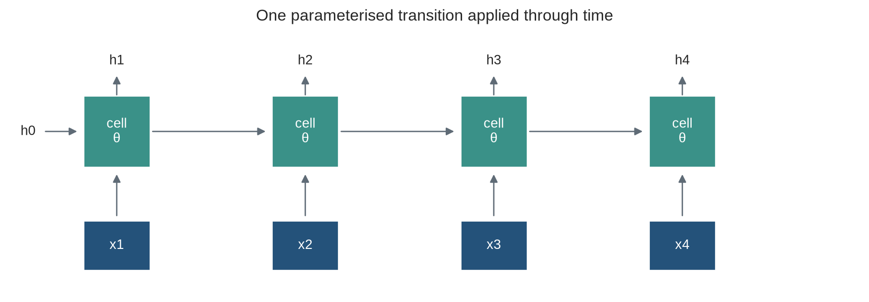
A recurrent network processes one position at a time. It combines the current input with a state produced at the previous position. The new state becomes a summary of the prefix seen so far. The same update rule is used at every position, so the model can process sequences longer or shorter than those used in one batch.
### State is memory with limited capacity
The hidden state is a finite vector. It can retain a useful feature of a long prefix, overwrite it with newer information, or encode several features in different coordinates. It cannot preserve every detail of an arbitrarily long sequence with fixed precision and fixed width.
```{python}
#| label: fig-rnn-unroll
#| fig-cap: "Unrolling exposes one recurrent cell reused across positions: each state receives the current input and the previous state."
#| fig-alt: "A left-to-right diagram shows four input vectors entering repeated recurrent cells. Hidden-state arrows connect the cells, and each cell uses the same parameters theta."
fig,ax=plt.subplots(figsize=(11.5,3.6)); ax.axis("off")
positions=range(4)
for t in positions:
    x=1+t*2.55
    ax.add_patch(Rectangle((x,.25),.9,.55,facecolor=blue,edgecolor="white")); ax.text(x+.45,.525,f"x{t+1}",ha="center",va="center",color="white")
    ax.add_patch(Rectangle((x,1.4),.9,.8,facecolor=teal,edgecolor="white")); ax.text(x+.45,1.8,"cell\nθ",ha="center",va="center",color="white")
    ax.add_patch(FancyArrowPatch((x+.45,.83),(x+.45,1.35),arrowstyle="-|>",mutation_scale=12,color=grey))
    ax.text(x+.45,2.55,f"h{t+1}",ha="center")
    ax.add_patch(FancyArrowPatch((x+.45,2.18),(x+.45,2.45),arrowstyle="-|>",mutation_scale=12,color=grey))
    if t>0: ax.add_patch(FancyArrowPatch((x-1.65,1.8),(x-.05,1.8),arrowstyle="-|>",mutation_scale=12,color=grey))
ax.text(.15,1.8,"h0",va="center"); ax.add_patch(FancyArrowPatch((.45,1.8),(.95,1.8),arrowstyle="-|>",mutation_scale=12,color=grey))
ax.set_xlim(0,11.5); ax.set_ylim(0,2.95); ax.set_title("One parameterised transition applied through time"); plt.show()
```
The unrolled picture contains several cells for explanation. The implementation stores one set of parameters. Parameter sharing is what turns a fixed update rule into a sequence model.
### The task determines when an output is available
A many-to-one model reads a sequence and produces one output, such as a final classification. A many-to-many model produces an output at each position, such as a tag for each item. An encoder reads a source sequence into states; a decoder produces a target sequence step by step. The same recurrent mechanism can appear in each arrangement, but the permitted direction of information differs.
For the delayed-copy task, the final output may use the final state. A causal next-item model at position $t$ may use only positions up to $t$. A bidirectional encoder may use both earlier and later positions, which is appropriate for labelling a complete observed sequence but invalid for real-time prediction.
### State updates make order explicit
If an early signal is useful, the recurrent update must preserve it. If a newer signal makes it irrelevant, the update should overwrite it. Plain recurrence has no explicit switch between these behaviours. Gated units add learned values between zero and one that regulate what is carried forward and what is replaced.
Level 1 established the operational purpose of state. Level 2 follows a delayed signal through a recurrence and its gates.
## Level 2 - Mechanics
### A plain recurrent cell combines input and prior state
For input $x_t$ and hidden state $h_{t-1}$, a basic recurrent update is
$$
h_t=\tanh(W_xx_t+W_hh_{t-1}+b).
$$
The input term introduces current evidence. The recurrent term carries transformed earlier evidence. Tanh bounds each coordinate, which can stabilise values but can also reduce gradients in saturated regions.
```{python}
x_values=np.array([1.,0.,0.,0.,0.])
W_x,W_h,b=1.0,.72,0.0
states=[]; h=0.0
for x in x_values:
    h=np.tanh(W_x*x+W_h*h+b); states.append(h)
print("inputs:",x_values)
print("states:",np.round(states,3))
```
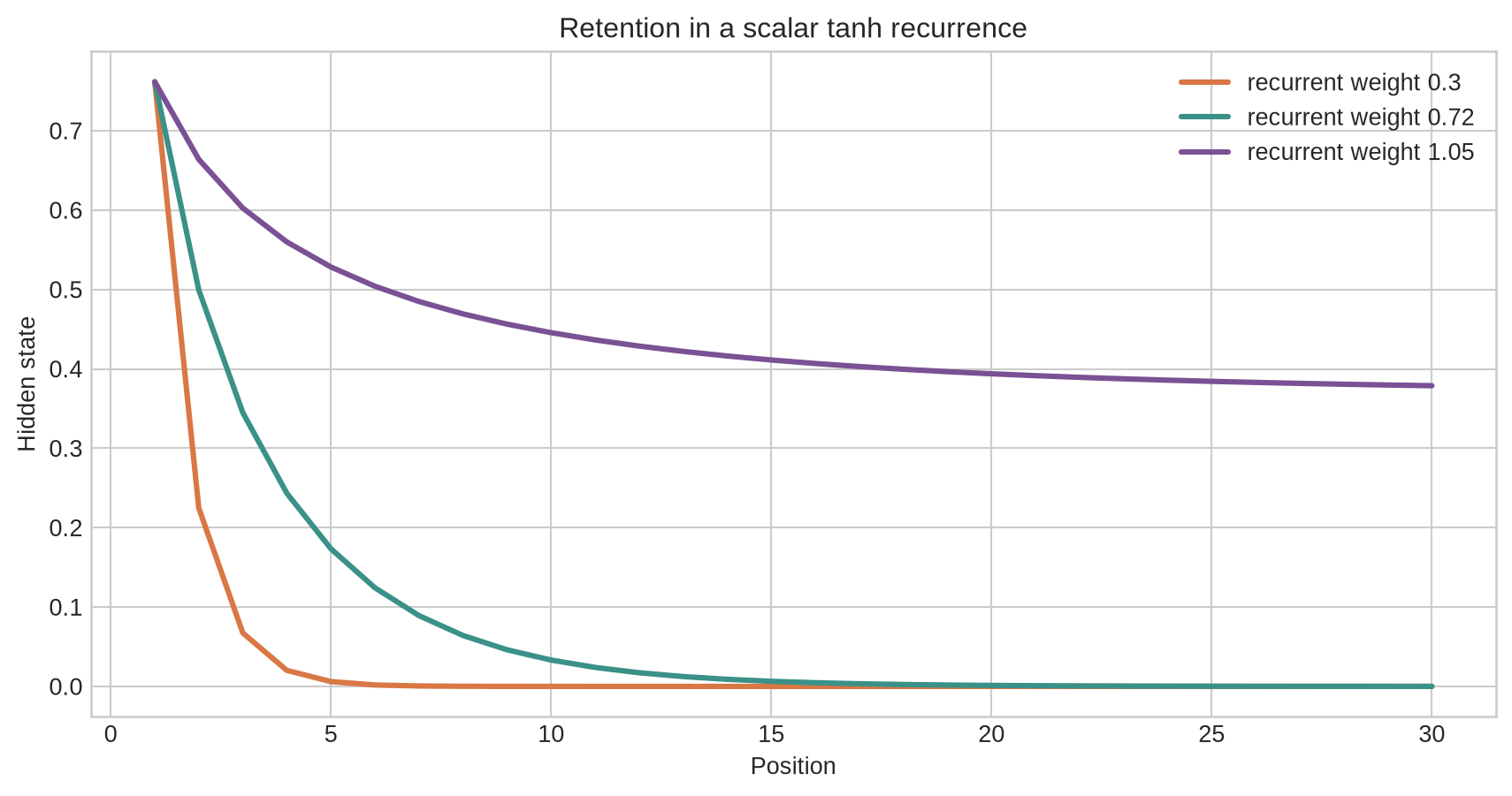
The first input enters the state. Later zero inputs do not restore the previous state; the recurrent multiplier and nonlinearity determine how rapidly the signal changes. A trained model has vector states and matrices, but the scalar calculation exposes the same dependence.
### Repeated transitions can erase or amplify a signal
```{python}
#| label: fig-state-retention
#| fig-cap: "The recurrent transition determines how much of an early signal remains available after later positions contain no new information."
#| fig-alt: "Three line charts show the hidden state after one initial signal and thirty zeros under recurrent multipliers 0.3, 0.72, and 1.05."
steps=30
fig,ax=plt.subplots(figsize=(9,4.8))
for recurrent_weight,colour in [(0.3,orange),(0.72,teal),(1.05,purple)]:
    h=0.; values=[]
    for x in [1.]+[0.]*(steps-1):
        h=np.tanh(x+recurrent_weight*h); values.append(h)
    ax.plot(range(1,steps+1),values,label=f"recurrent weight {recurrent_weight}",color=colour,linewidth=2.3)
ax.set_xlabel("Position"); ax.set_ylabel("Hidden state"); ax.set_title("Retention in a scalar tanh recurrence"); ax.legend(); plt.tight_layout(); plt.show()
```
The values do not follow a pure power because tanh is nonlinear. The comparison nevertheless shows the mechanism: a state that is repeatedly contracted loses early evidence. A larger recurrent weight can retain more signal but may also create unstable dynamics in other regions of state space.
### Gates create a direct controlled path
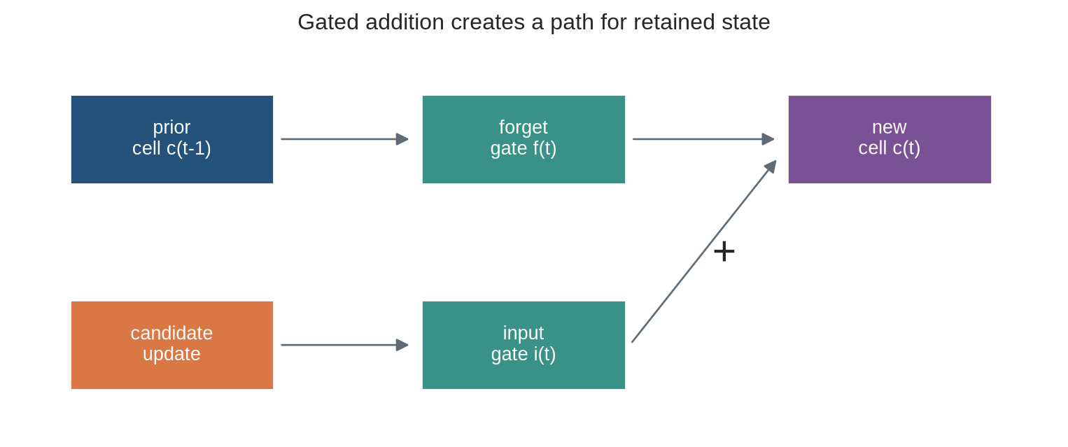
An LSTM maintains a cell state $c_t$ and uses gates to regulate its update [@hochreiter1997lstm]. In a simplified form,
$$
c_t=f_t\odot c_{t-1}+i_t\odot \tilde c_t,
$$
where $f_t$ is the forget gate, $i_t$ the input gate, and $\tilde c_t$ a candidate update. Values near one preserve or write; values near zero block the corresponding contribution. An output gate determines how the cell becomes the visible hidden state.
```{python}
#| label: fig-gated-update
#| fig-cap: "Forget and input gates separate retention from replacement: the cell state is a weighted combination of the prior state and a proposed update."
#| fig-alt: "A diagram shows prior cell state passing through a forget gate and a candidate update passing through an input gate; both paths add to the new cell state."
fig,ax=plt.subplots(figsize=(10,3.8)); ax.axis("off")
boxes=[(.5,2.2,"prior\ncell c(t-1)",blue),(3.0,2.2,"forget\ngate f(t)",teal),(5.6,2.2,"new\ncell c(t)",purple),(.5,.55,"candidate\nupdate",orange),(3.0,.55,"input\ngate i(t)",teal)]
for x,y,label,colour in boxes:
    ax.add_patch(Rectangle((x,y),1.45,.72,facecolor=colour,edgecolor="white")); ax.text(x+.725,y+.36,label,ha="center",va="center",color="white")
for start,end in [((1.98,2.56),(2.94,2.56)),((4.48,2.56),(5.54,2.56)),((1.98,.91),(2.94,.91)),((4.48,.91),(5.54,2.42))]:
    ax.add_patch(FancyArrowPatch(start,end,arrowstyle="-|>",mutation_scale=14,color=grey))
ax.text(5.15,1.55,"+",fontsize=22,ha="center"); ax.set_xlim(.1,7.5); ax.set_ylim(.2,3.35); ax.set_title("Gated addition creates a path for retained state"); plt.show()
```
A GRU uses a related update gate to interpolate between a previous hidden state and a candidate state [@cho2014gru]. Different gated formulations make different parameter and state choices, but each tries to give optimisation a route through time that plain recurrence lacks.
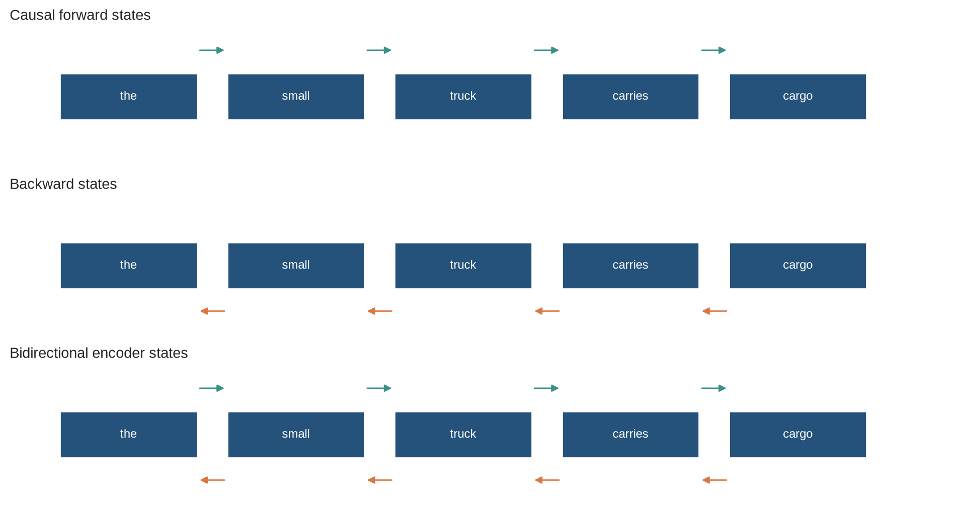
### Bidirectionality uses information from both sides
```{python}
#| label: fig-processing-directions
#| fig-cap: "Causal recurrence exposes only earlier positions; bidirectional encoding combines a forward and backward summary at each position."
#| fig-alt: "A three-row diagram shows five tokens. Forward arrows move left to right, backward arrows move right to left, and bidirectional states combine both arrows at every token."
tokens=["the","small","truck","carries","cargo"]
fig,axes=plt.subplots(3,1,figsize=(10,5.4),sharex=True)
for ax,title in zip(axes,["Causal forward states","Backward states","Bidirectional encoder states"]):
    ax.set_title(title,loc="left",fontsize=11); ax.axis("off"); ax.set_xlim(-.3,5.3); ax.set_ylim(-.2,1.2)
    for i,token in enumerate(tokens):
        ax.add_patch(Rectangle((i,.25),.82,.48,facecolor=blue,edgecolor="white")); ax.text(i+.41,.49,token,ha="center",va="center",color="white",fontsize=9)
for i in range(4): axes[0].add_patch(FancyArrowPatch((i+.82,.97),(i+1,.97),arrowstyle="-|>",mutation_scale=11,color=teal))
for i in range(4): axes[1].add_patch(FancyArrowPatch((i+1,.02),(i+.82,.02),arrowstyle="-|>",mutation_scale=11,color=orange))
for i in range(4):
    axes[2].add_patch(FancyArrowPatch((i+.82,.97),(i+1,.97),arrowstyle="-|>",mutation_scale=11,color=teal))
    axes[2].add_patch(FancyArrowPatch((i+1,.02),(i+.82,.02),arrowstyle="-|>",mutation_scale=11,color=orange))
plt.tight_layout(); plt.show()
```
The backward pass is available only after the complete sequence is observed. It cannot be used unchanged for a system that must produce a prediction before future events arrive. Masking and sequence boundaries are part of this direction contract.
### Encoder-decoder models expose a fixed-vector bottleneck
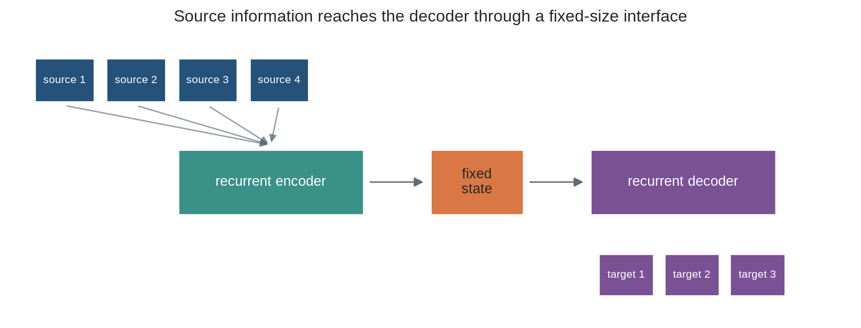
An early sequence-to-sequence encoder maps a source sequence to a final state. A decoder conditions each target step on that one state and on earlier target outputs. This permits variable source and target lengths, but it asks a fixed-width vector to make source details available across all decoding steps.
```{python}
#| label: fig-fixed-vector-bottleneck
#| fig-cap: "A fixed-vector encoder-decoder must compress every relevant source detail into one state before the decoder begins."
#| fig-alt: "A source sequence flows through an encoder into one narrow context vector, then into a decoder that produces a target sequence. The central vector is highlighted as a bottleneck."
fig,ax=plt.subplots(figsize=(11,3.8)); ax.axis("off")
for i,label in enumerate(["source 1","source 2","source 3","source 4"]):
    ax.add_patch(Rectangle((.3+i*.85,2.4),.7,.48,facecolor=blue,edgecolor="white")); ax.text(.65+i*.85,2.64,label,ha="center",va="center",fontsize=8,color="white")
ax.add_patch(Rectangle((2.0,1.15),2.2,.72,facecolor=teal,edgecolor="white")); ax.text(3.1,1.51,"recurrent encoder",ha="center",va="center",color="white")
ax.add_patch(Rectangle((5.0,1.15),1.1,.72,facecolor=orange,edgecolor="white")); ax.text(5.55,1.51,"fixed\nstate",ha="center",va="center")
ax.add_patch(Rectangle((6.9,1.15),2.2,.72,facecolor=purple,edgecolor="white")); ax.text(8.0,1.51,"recurrent decoder",ha="center",va="center",color="white")
for i in range(4): ax.add_patch(FancyArrowPatch((.65+i*.85,2.36),(3.1,1.92),arrowstyle="-|>",mutation_scale=11,color=grey,alpha=.65))
for start,end in [((4.25,1.51),(4.95,1.51)),((6.15,1.51),(6.85,1.51))]: ax.add_patch(FancyArrowPatch(start,end,arrowstyle="-|>",mutation_scale=14,color=grey))
for i,label in enumerate(["target 1","target 2","target 3"]):
    ax.add_patch(Rectangle((7.0+i*.78,.25),.65,.46,facecolor=purple,edgecolor="white")); ax.text(7.325+i*.78,.48,label,ha="center",va="center",fontsize=8,color="white")
ax.set_xlim(0,10); ax.set_ylim(0,3.2); ax.set_title("Source information reaches the decoder through a fixed-size interface"); plt.show()
```
The bottleneck is not a statement that the final state contains no useful information. It is a constraint on access: every decoder decision must rely on the same compressed source summary. Chapter 19 examines the mechanism that lets a decoder construct a different source-dependent context at each step.
Level 2 described recurrent operation and its practical pressure points. Level 3 derives the temporal gradient and implements recurrent modules.
## Level 3 - Mathematics & Code
### Unrolling turns recurrence into a deep computation graph
For the plain recurrence $h_t=\phi(W_xx_t+W_hh_{t-1}+b)$, a final loss $L$ depends on $h_1$ through every later state. The gradient with respect to an earlier state contains products of Jacobians:
$$
\frac{\partial L}{\partial h_t}=
\frac{\partial L}{\partial h_T}
\prod_{k=t+1}^{T}\frac{\partial h_k}{\partial h_{k-1}}.
$$
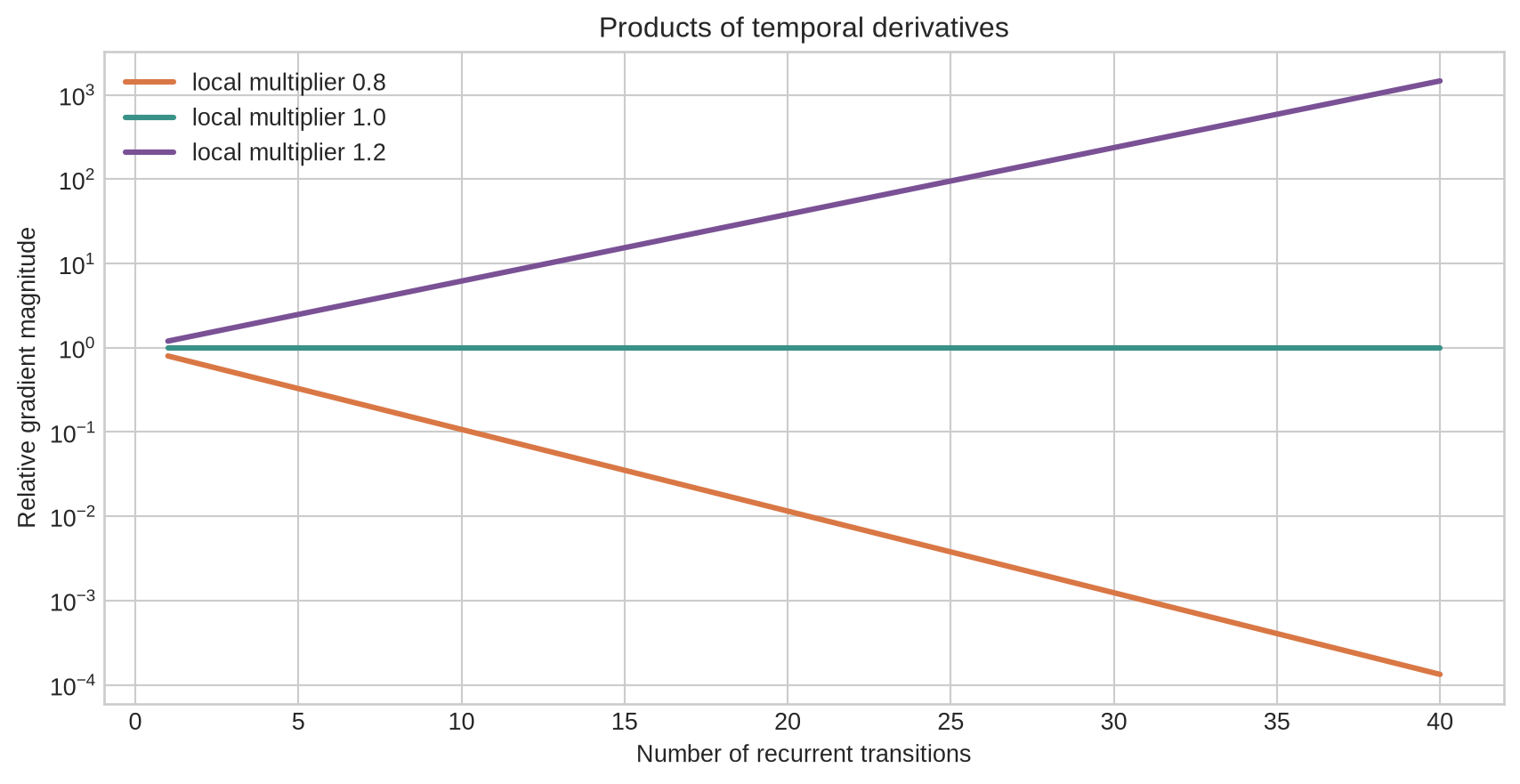
For a scalar linear recurrence with multiplier $a$, the product is $a^{T-t}$. If $|a|<1$, it shrinks exponentially; if $|a|>1$, it grows exponentially. In nonlinear networks, each factor also contains activation derivatives and matrix directions.
```{python}
#| label: fig-temporal-gradients
#| fig-cap: "Backpropagation through time multiplies one local derivative per step, so a small contraction or expansion compounds with sequence length."
#| fig-alt: "A log-scale plot shows gradient magnitude across one to forty time steps for local derivative multipliers 0.8, 1.0, and 1.2."
steps=np.arange(1,41)
fig,ax=plt.subplots(figsize=(9,4.7))
for derivative,colour in [(0.8,orange),(1.0,teal),(1.2,purple)]:
    ax.plot(steps,derivative**steps,label=f"local multiplier {derivative}",color=colour,linewidth=2.3)
ax.set_yscale("log"); ax.set_xlabel("Number of recurrent transitions"); ax.set_ylabel("Relative gradient magnitude")
ax.set_title("Products of temporal derivatives"); ax.legend(); plt.tight_layout(); plt.show()
```
Backpropagation through time applies the same chain rule introduced in Chapter 4 to the unrolled graph. @pascanu2013difficulty analyse the vanishing and exploding gradient problems in recurrent networks and discuss gradient clipping as one response to explosions. Clipping limits update magnitude; it does not restore information lost through sustained contraction.
### Gated cell equations expose retention paths
One common LSTM parameterisation is
$$
\begin{aligned}
f_t&=\sigma(W_f[x_t,h_{t-1}]+b_f),\\
i_t&=\sigma(W_i[x_t,h_{t-1}]+b_i),\\
\tilde c_t&=\tanh(W_c[x_t,h_{t-1}]+b_c),\\
c_t&=f_t\odot c_{t-1}+i_t\odot\tilde c_t,\\
o_t&=\sigma(W_o[x_t,h_{t-1}]+b_o),\\
h_t&=o_t\odot\tanh(c_t).
\end{aligned}
$$
The forget gate directly multiplies the prior cell. When $f_t$ remains near one and the remaining terms are controlled, a component of $c_{t-1}$ can persist across many steps. This is a learned possibility, not a guarantee that a fitted model will use long-range information.
```{python}
forget_values=np.array([.15,.55,.92])
initial_cell=1.0
for forget in forget_values:
    retained=initial_cell*forget**20
    print(f"forget gate {forget:.2f}: cell contribution after 20 steps = {retained:.5f}")
```
The calculation isolates one path by setting new candidate contributions aside. In a real LSTM, input, output, and forget gates depend on inputs and hidden state at every position; the full dynamics can retain, overwrite, or mix information in more complex ways.
### Framework modules preserve the sequence axis
```{python}
import torch
from torch import nn

torch.manual_seed(18)
inputs=torch.randn(3,5,4)  # batch, positions, embedding features
gru=nn.GRU(input_size=4,hidden_size=6,batch_first=True)
outputs,final_state=gru(inputs)
bidirectional=nn.GRU(input_size=4,hidden_size=6,batch_first=True,bidirectional=True)
bi_outputs,bi_final=bidirectional(inputs)
print("forward outputs:",tuple(outputs.shape),"final state:",tuple(final_state.shape))
print("bidirectional outputs:",tuple(bi_outputs.shape),"final state:",tuple(bi_final.shape))
```
The forward GRU returns one six-dimensional output at each of five positions and one final state per batch item. The bidirectional output concatenates forward and backward features, giving width twelve at each position. Framework shape validity does not establish causal validity: a bidirectional output includes future positions by construction.
### Variable lengths require packing or masks
```{python}
lengths=torch.tensor([5,3,2])
sequence=torch.randn(3,5,4)
packed=nn.utils.rnn.pack_padded_sequence(sequence,lengths,batch_first=True,enforce_sorted=False)
packed_output,packed_final=gru(packed)
unpacked,returned_lengths=nn.utils.rnn.pad_packed_sequence(packed_output,batch_first=True)
print("unpacked shape:",tuple(unpacked.shape),"returned lengths:",returned_lengths.tolist())
```
Packing prevents recurrent updates from treating padded positions as observations. A masking implementation must provide equivalent protection. The final-state convention, padding side, sorted order, and truncation rule should be recorded because they change which state represents each sequence.
Level 3 has connected temporal derivatives and tensor shapes to recurrent computation. Level 4 considers sequence models as training and systems objects, and marks the precise transition to attention.
## Level 4 - Research & Systems
### Recurrent models have sequential depth
A recurrent layer has one transition per position. Within a position, matrix multiplications can use accelerator parallelism across batch items and hidden dimensions. Across positions, the next state depends on the preceding state. This dependency limits training and inference parallelism over sequence length.
Padding creates wasted recurrent steps when sequence lengths vary. Bucketing similar lengths, packing valid positions, and truncating or chunking streams can reduce this waste. Each choice changes batching, memory use, latency, and the span over which gradients and state can propagate.
### Truncated backpropagation creates an explicit learning horizon
Long streams are often divided into segments. Hidden state may be carried from one segment to the next while gradients are detached at the boundary. The forward state then contains older information, but parameter updates receive no gradient through the detached history. This is a substantive training assumption, not only a memory optimisation.
An implementation should state segment length, overlap, state-reset conditions, detach points, and whether evaluation uses the same state policy. Leakage can arise if a state carries information across independent sequences or across train, validation, and test boundaries.
### Gates improve optimisation but do not remove all sequence limits
LSTM and GRU units address plain recurrent gradient paths by offering additive or interpolating memory updates [@hochreiter1997lstm; @cho2014gru]. They still have finite state width, may forget information, and process positions sequentially. Gating also adds parameter matrices and elementwise operations, so shorter sequences or smaller states can remain more efficient even when long dependency capacity is desirable.
Gate values are diagnostics, not explanations by themselves. A forget gate near one at one position does not show which information was preserved or whether it affected the output. Useful analysis connects controlled changes in input or state to later predictions under a declared task.
### Encoder-decoder bottlenecks motivated attention
Early encoder-decoder systems encoded a variable-length source in one fixed-length vector [@cho2014gru]. This is workable for short patterns but creates a constrained interface as source length and target requirements grow. @bahdanau2015attention introduced a learned alignment mechanism that lets a decoder form a different weighted context from encoder states at each output step.
The historical motivation should not be read as a claim that attention automatically solves long-context reliability, memory, or computation. It changes the access pattern: source states become separately available to a decoder. Chapter 19 derives that weighted retrieval operation. Chapters 20–22 then develop self-attention, positional information, and the Transformer block.
### Sequence direction is a deployment constraint
Bidirectional encoders can use future context and are therefore appropriate for retrospective labelling, document classification, and some offline analysis. Autoregressive generation and streaming alerts require causal processing. A model trained with a bidirectional encoder can report optimistic validation results if its deployment target lacks future observations.
The representation contract must state which positions are visible at prediction time. It should also state clock definitions, ordering rules for tied events, missing-position treatment, padding, resets, and whether a hidden state can cross a user, document, session, or device boundary.
### A sequence-model audit connects information flow to evaluation
An audit should record:
- the item encoding, sequence order, time unit, and treatment of tied or missing events;
- the task arrangement: many-to-one, many-to-many, encoder-decoder, causal, or bidirectional;
- hidden-state width, cell type, layers, dropout, initial-state rule, and parameter count;
- padding, masks, packing, bucketing, truncation, segment length, and reset policy;
- gradient norms by time span, clipping frequency, non-finite values, and gate or state summaries where relevant;
- train, validation, and test boundaries for stateful streams;
- latency, throughput, sequence-length distribution, and peak activation memory;
- accuracy and calibration by dependency length, position, sequence length, and relevant population or domain group.
The final point is often neglected. A model can achieve strong average performance by relying mainly on recent information while failing precisely when the target depends on a long earlier span.
## Common misconceptions
- **Embeddings already model order.** Lookup preserves position but does not combine positions.
- **A recurrent state stores the full sequence.** It is a fixed-width learned summary.
- **Unrolling creates separate parameters for each position.** The same recurrent weights are reused.
- **A stable hidden value proves a stable gradient.** Forward-state retention and backward derivatives are related but distinct.
- **A recurrent multiplier below one always causes vanishing gradients at the same rate.** Activation derivatives and matrix directions also enter the product.
- **Gradient clipping solves long-term dependency learning.** It limits exploding updates but does not reverse contraction.
- **LSTMs never forget.** Their gates can preserve, overwrite, or block information.
- **A gate value explains a prediction.** It describes one update factor, not causal use of a feature.
- **Bidirectional models are stronger causal models.** They use future observations unavailable in causal deployment.
- **Padding values are harmless in recurrence.** Unmasked recurrence can update state from padding.
- **Carrying state across batches is always efficient.** It can leak information across independent sequences or splits.
- **The encoder final state is a complete source representation.** It is one fixed-width interface with limited access capacity.
- **Attention removes sequence order automatically.** Attention requires an explicit treatment of position, addressed in Chapter 21.
- **Recurrent networks cannot process long sequences.** They can, but optimisation, memory, latency, and dependency quality must be measured.
## Exercises
1. Give two sequences with identical sums of embedding vectors but different order-dependent meanings or targets.
2. Write the shape of a batch of 32 sequences, length 100, embedding width 256 before and after a forward GRU with hidden width 512.
3. Calculate five scalar recurrent updates for $h_t=\tanh(x_t+0.6h_{t-1})$ with one initial signal followed by zeros.
4. Repeat the calculation with a recurrent multiplier of 1.1 and compare the forward states.
5. Explain why both calculations are insufficient to establish trainability.
6. Derive the gradient product for a scalar linear recurrence over ten steps.
7. Plot the products for local derivatives 0.9, 1.0, and 1.1 over 100 steps.
8. Explain the roles of the forget, input, and output gates in an LSTM.
9. Calculate the retained contribution of an initial cell value under three constant forget-gate values.
10. Compare a GRU update gate with the LSTM's separate forget and input gates.
11. Implement a causal GRU and verify that permuting future positions leaves an earlier output unchanged.
12. Implement a bidirectional GRU and show why that test no longer holds.
13. Use packed sequences with lengths 6, 4, and 1 and verify that padded positions do not create valid outputs.
14. Define a state-reset policy for independent user sessions and explain the leakage risk of violating it.
15. Design a delayed-copy dataset with dependency lengths from 1 to 100 and report accuracy by length.
16. Implement truncated backpropagation through time and state its gradient horizon.
17. Compare full and truncated gradients on a short sequence where both are feasible.
18. Draw the information available at position four for causal, backward, and bidirectional processing.
19. Explain why a fixed encoder vector can constrain a long source-to-target task.
20. Specify the metadata required to reproduce one sequence-model prediction in a streaming system.
21. Estimate how doubling sequence length changes the number of recurrent transitions and saved states for one layer.
22. Design an evaluation that detects whether a model relies on the first, middle, or final portion of a sequence.
## Summary
Sequence models must make earlier and later positions interact. Recurrent networks do this by carrying a hidden state through an ordered sequence with shared parameters. The state is a learned prefix summary, not a complete record. It can retain, overwrite, or mix information according to the recurrent transition and, in gated models, learned control values.
Unrolling a recurrent network produces a computation graph whose gradient contains products of temporal derivatives. These products can contract or expand sharply with sequence length. LSTMs and GRUs create more direct controlled paths through state, but they retain finite memory, sequential dependence, and optimisation limits.
Bidirectional encoders use both sides of a position and therefore require a complete sequence. Encoder-decoder systems show a further constraint when one final source state must support all target decisions. The next chapter introduces attention as a learned way to construct a different source-dependent context at each output step.
## Looking ahead
[Chapter 19](19-attention.qmd) introduces attention. It replaces the fixed-vector access pattern by comparing a current query with a collection of source representations, converting the resulting scores into weights, and forming a weighted retrieval vector.
## Further reading
The simple recurrent network is developed by @elman1990. The original LSTM architecture is described by @hochreiter1997lstm, and the GRU encoder-decoder by @cho2014gru. Temporal gradient problems are analysed by @pascanu2013difficulty. The fixed-vector encoder-decoder limitation and its attention-based response are developed by @bahdanau2015attention.