---
title: "Activation Functions and Non-linearity"
subtitle: "Why depth needs a change of shape"
---
## The problem
Chapter 6 showed how one layer can produce several values for the next. It may seem that adding further layers would automatically make the network able to describe more complicated patterns. It does not. If each layer only multiplies, adds, and passes its result on, the full stack still behaves like one straight-rule calculation.
An activation function changes a value before the next layer receives it. That small operation is what lets a network use one simple rule in one part of its input range and another elsewhere.
### The running calculations
The first example continues the layer calculation from Chapter 6. Its pre-activation vector is
$$
z=(2,1.5,-1.5).
$$
Applying ReLU gives $h=(2,1.5,0)$. We will begin by following this change one value at a time.
A second, one-dimensional example will show how changing individual values can produce a curve with different slopes.
## Level 1 - Intuition
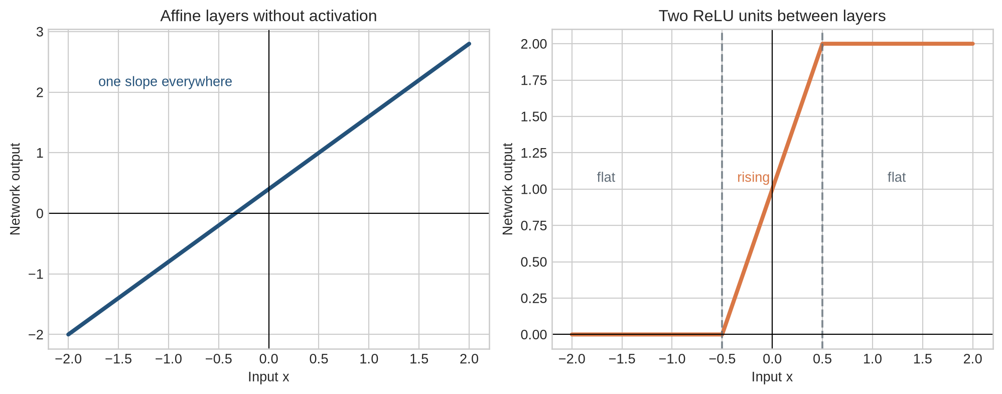
Read the two panels from left to right. The first model has several calculations but one straight input-output relationship. In the second, ReLU switches individual values on or off as the input changes, creating separate regions.
### More layers do not help if every layer follows the same straight rule
An affine layer can rescale and shift its input. A second affine layer can do the same, but the combined result remains one straight relationship. The intermediate layer may contain more values, yet the final output has not acquired a bend.
An activation is inserted between layers to change that relationship. Each unit first calculates its pre-activation. ReLU keeps a positive value and replaces a negative value with zero. As the input changes, different units cross zero at different points. The network can therefore follow different straight segments in different regions.
```{python}
#| label: fig-nonlinearity-intuition
#| fig-cap: "Without an activation, two affine layers produce one straight relationship; ReLU units allow the slope to change across input regions."
#| fig-alt: "Two panels compare a straight affine input-output line with a piecewise-linear ReLU network that is flat, then rises, then becomes flat again."
import numpy as np
import matplotlib.pyplot as plt

plt.style.use("seaborn-v0_8-whitegrid")
blue, teal, orange, grey = "#24527a", "#3a9188", "#d97745", "#5f6b76"

x_grid = np.linspace(-2, 2, 401)
affine_y = 1.2 * x_grid + 0.4
relu_network_y = np.maximum(0, 2 * x_grid + 1) - np.maximum(0, 2 * x_grid - 1)

fig, axes = plt.subplots(1, 2, figsize=(10.5, 4.2), sharex=True)
axes[0].plot(x_grid, affine_y, color=blue, linewidth=3)
axes[0].set_title("Affine layers without activation")
axes[0].text(-1.7, 2.1, "one slope everywhere", color=blue)

axes[1].plot(x_grid, relu_network_y, color=orange, linewidth=3)
axes[1].axvline(-0.5, color=grey, linestyle="--", alpha=0.7)
axes[1].axvline(0.5, color=grey, linestyle="--", alpha=0.7)
axes[1].text(-1.75, 1.05, "flat", color=grey)
axes[1].text(-0.35, 1.05, "rising", color=orange)
axes[1].text(1.15, 1.05, "flat", color=grey)
axes[1].set_title("Two ReLU units between layers")

for ax in axes:
    ax.axhline(0, color="black", linewidth=0.8)
    ax.axvline(0, color="black", linewidth=0.8)
    ax.set_xlabel("Input x")
    ax.set_ylabel("Network output")
plt.tight_layout()
plt.show()
```
The left panel has one slope across the full input range. The right panel has three regions. Below $-0.5$, both ReLU units return zero. Between $-0.5$ and $0.5$, one unit is active and the output rises. Above $0.5$, both are active and their slopes cancel, leaving an output of two. The network is still made from simple calculations, but the activation lets them join into a bent relationship.
::: {.concept-box .concept-core #concept-activation-function data-term="Activation function" data-domain="Foundations"}
**Activation function.** A fixed rule applied to a layer's pre-activation values before they are passed on. It changes the shape of the relationship the full network can represent; ReLU, for example, replaces negative values with zero.
:::
### An activation acts on values, not on substantive meaning
In a dense hidden layer, the same activation function is normally applied to every coordinate. If $z=(2,1.5,-1.5)$, ReLU processes the three numbers independently and returns $(2,1.5,0)$. It does not know that one coordinate may describe distance or that another may represent prior participation. The weights create the pre-activations; the activation applies a fixed numerical rule.
### Hidden activations and output transformations
An activation between hidden layers changes what the network can represent. A transformation at the output can have another job: sigmoid maps one score to a value between zero and one, and softmax converts several scores into values that sum to one. The different output contracts are taken up when the book returns to prediction tasks.
The main conclusion at this level is specific: hidden activations prevent a deep network from collapsing into one affine map. The next level follows ReLU through the running vector.
## Level 2 - Mechanics
### The activation step has three parts
For a hidden layer, the forward calculation can be separated into three operations:
1. calculate the pre-activation $z=Wx+b$;
2. apply an activation independently to each coordinate, $h_j=\phi(z_j)$;
3. pass the resulting vector $h$ to the next layer.
For the Chapter 6 vector, ReLU gives
$$
\operatorname{ReLU}(2)=2,\qquad
\operatorname{ReLU}(1.5)=1.5,\qquad
\operatorname{ReLU}(-1.5)=0.
$$
The third unit is not removed from the network. Its output is zero for this observation. The same unit may be active for another observation whose pre-activation is positive.
## Level 3 - Mathematics & Code
The running vector established the elementwise operation. This level compares several activation rules, relates them to the gradients introduced in Chapter 4, and then writes out why the activation stops stacked layers from collapsing into one affine function.
### Common activations transform the same input differently
Four functions will be compared throughout this chapter:
$$
\begin{aligned}
\operatorname{ReLU}(z) &= \max(0,z),\\
\sigma(z) &= \frac{1}{1+e^{-z}},\\
\tanh(z) &= \frac{e^z-e^{-z}}{e^z+e^{-z}},\\
\operatorname{GELU}(z) &= z\Phi(z),
\end{aligned}
$$
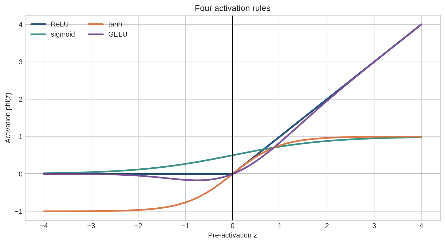
where $\Phi(z)$ is the standard normal cumulative distribution function. ReLU discards negative values. Sigmoid compresses all values into $(0,1)$. Tanh compresses them into $(-1,1)$. GELU attenuates negative inputs smoothly and approaches the identity for sufficiently positive inputs [@hendrycks2016gelu].
```{python}
#| label: fig-activation-comparison
#| fig-cap: "ReLU, sigmoid, tanh, and GELU apply different transformations to the same pre-activation."
#| fig-alt: "A line chart compares four activation functions from negative four to positive four, showing their different ranges, smoothness, and treatment of negative inputs."
from math import erf

def sigmoid_np(z):
    return 1 / (1 + np.exp(-z))

def gelu_np(z):
    erf_values = np.vectorize(erf)(z / np.sqrt(2))
    return 0.5 * z * (1 + erf_values)

z_plot = np.linspace(-4, 4, 500)
fig, ax = plt.subplots(figsize=(9, 5))
ax.plot(z_plot, np.maximum(0, z_plot), label="ReLU", color=blue, linewidth=2.7)
ax.plot(z_plot, sigmoid_np(z_plot), label="sigmoid", color=teal, linewidth=2.4)
ax.plot(z_plot, np.tanh(z_plot), label="tanh", color=orange, linewidth=2.4)
ax.plot(z_plot, gelu_np(z_plot), label="GELU", color="#7a5195", linewidth=2.4)
ax.axhline(0, color="black", linewidth=0.8)
ax.axvline(0, color="black", linewidth=0.8)
ax.set_xlabel("Pre-activation z")
ax.set_ylabel("Activation phi(z)")
ax.set_title("Four activation rules")
ax.legend(ncol=2)
plt.tight_layout()
plt.show()
```
The graph shows why the name of an activation is not enough to describe its effect. ReLU and GELU are unbounded above, whereas sigmoid and tanh approach fixed limits. Tanh is centred around zero; sigmoid is not. ReLU has a sharp corner at zero; sigmoid, tanh, and GELU are smooth. These differences affect both the values sent forward and the gradients sent backward.
For a few representative inputs:
| $z$ | ReLU | sigmoid | tanh | GELU |
|---:|---:|---:|---:|---:|
| -2.0 | 0.000 | 0.119 | -0.964 | -0.046 |
| -0.5 | 0.000 | 0.378 | -0.462 | -0.154 |
| 0.0 | 0.000 | 0.500 | 0.000 | 0.000 |
| 0.5 | 0.500 | 0.622 | 0.462 | 0.346 |
| 2.0 | 2.000 | 0.881 | 0.964 | 1.954 |
The table should be read row by row. At $z=-2$, ReLU transmits no value, while GELU transmits a small negative value and sigmoid returns a positive value because its output range starts at zero. At $z=2$, ReLU is exactly linear, GELU is close to linear, and the bounded functions are already flattening.
### The backward pass uses the local slope
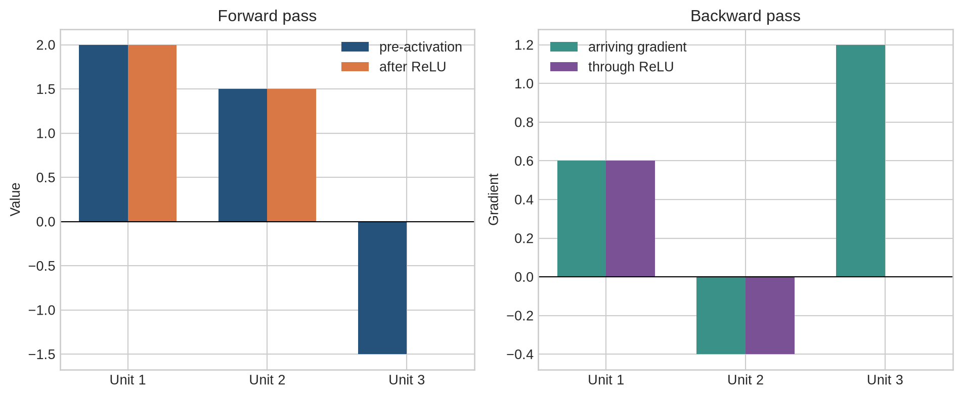
Backpropagation multiplies the gradient arriving from the next operation by the activation's derivative. ReLU therefore behaves as a gate away from zero: positive pre-activations pass the gradient; negative pre-activations return zero. With upstream gradient
$$
g_h=(0.6,-0.4,1.2),
$$
the running example gives
$$
g_z=g_h\odot(1,1,0)=(0.6,-0.4,0).
$$
The third unit receives no gradient through ReLU for this observation. This is an observation-specific statement. A batch containing positive pre-activations for that unit can still update its incoming weights.
```{python}
#| label: fig-relu-gate
#| fig-cap: "ReLU uses the sign of the pre-activation in both the forward and backward passes."
#| fig-alt: "Three units show positive, positive, and negative pre-activations; ReLU preserves the first two outputs and gradients but sets the third output and gradient to zero."
z_run = np.array([2.0, 1.5, -1.5])
upstream = np.array([0.6, -0.4, 1.2])
h_run = np.maximum(0, z_run)
grad_z = upstream * (z_run > 0)

fig, axes = plt.subplots(1, 2, figsize=(10, 4.2))
positions = np.arange(3)
width = 0.35
axes[0].bar(positions - width/2, z_run, width, label="pre-activation", color=blue)
axes[0].bar(positions + width/2, h_run, width, label="after ReLU", color=orange)
axes[0].set_title("Forward pass")
axes[0].set_ylabel("Value")
axes[0].legend()
axes[1].bar(positions - width/2, upstream, width, label="arriving gradient", color=teal)
axes[1].bar(positions + width/2, grad_z, width, label="through ReLU", color="#7a5195")
axes[1].set_title("Backward pass")
axes[1].set_ylabel("Gradient")
axes[1].legend()
for ax in axes:
    ax.axhline(0, color="black", linewidth=0.8)
    ax.set_xticks(positions, ["Unit 1", "Unit 2", "Unit 3"])
plt.tight_layout()
plt.show()
```
The two panels describe the same mask. Unit 3 is inactive in the forward pass and blocks this observation's gradient in the backward pass. Units 1 and 2 preserve their values and pass the arriving gradients unchanged.
### Activation choice depends on where the function is used
ReLU and GELU are common hidden activations because their positive side does not approach a fixed upper bound. Sigmoid is useful when a scalar output must lie between zero and one, and it also appears inside gates. Tanh remains useful where a bounded, zero-centred state is wanted. Softmax is usually applied across a vector of output scores, rather than independently to each coordinate. No single activation has the same role in every location.
### Two affine layers collapse into one
Let the first layer be
$$
z_1=W_1x+b_1
$$
and the second
$$
y=W_2z_1+b_2.
$$
Substitution gives
$$
\begin{aligned}
y &= W_2(W_1x+b_1)+b_2\\
&= (W_2W_1)x+(W_2b_1+b_2).
\end{aligned}
$$
Define $W_*=W_2W_1$ and $b_*=W_2b_1+b_2$. Then $y=W_*x+b_*$. The dimensions of the intermediate layer may be large, but the represented function remains affine.
With an activation,
$$
y=W_2\phi(W_1x+b_1)+b_2,
$$
the same simplification is generally unavailable because $\phi(W_1x+b_1)$ cannot be replaced by a fixed matrix multiplying $x$. For ReLU, the active units depend on the input. Within a region where the active set stays fixed, the network is affine; crossing a ReLU threshold changes the effective affine map.
### The one-dimensional network is piecewise affine
The running scalar network can be written in three regions:
$$
y(x)=
\begin{cases}
0, & x<-0.5,\\
2x+1, & -0.5\leq x<0.5,\\
2, & x\geq0.5.
\end{cases}
$$
At $x=-1$, both hidden pre-activations are non-positive and $y=0$. At $x=0$, the first is active, the second inactive, and $y=1$. At $x=1$, both are active and $y=3-1=2$. This calculation explains the three regions shown in the Level 1 figure.
```{python}
# Verify the piecewise calculation directly.
def small_relu_network(x):
    hidden = np.maximum(0, np.array([2*x + 1, 2*x - 1]))
    return hidden[0] - hidden[1]

for value in [-1.0, 0.0, 1.0]:
    print(f"x={value:>4.1f}, y={small_relu_network(value):.1f}")
```
The outputs are 0, 1, and 2. They agree with the region-specific formula. The code contains no special cases because ReLU creates the regions through its elementwise rule.
### Derivatives determine gradient transmission
Away from points where a derivative is undefined, the common derivatives are
$$
\begin{aligned}
\operatorname{ReLU}'(z) &= \begin{cases}0&z<0\\1&z>0,\end{cases}\\
\sigma'(z) &= \sigma(z)[1-\sigma(z)],\\
\tanh'(z) &= 1-\tanh^2(z),\\
\operatorname{GELU}'(z) &= \Phi(z)+z\varphi(z),
\end{aligned}
$$
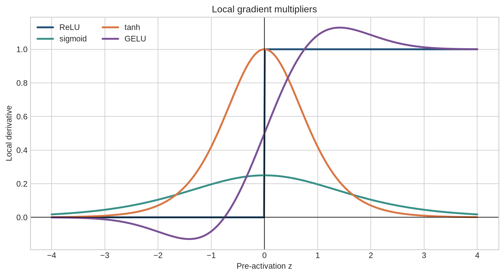
where $\varphi(z)$ is the standard normal density. ReLU is not differentiable at zero; software libraries assign a conventional subgradient there, commonly zero. This single-point convention is different from ReLU's zero derivative over the entire negative half-line.
```{python}
#| label: fig-activation-derivatives
#| fig-cap: "Activation derivatives determine how much of an upstream gradient is transmitted locally."
#| fig-alt: "A line chart compares ReLU, sigmoid, tanh, and GELU derivatives. Sigmoid and tanh approach zero at large magnitudes; ReLU is zero for negative inputs and one for positive inputs."
normal_pdf = np.exp(-0.5 * z_plot**2) / np.sqrt(2 * np.pi)
normal_cdf = 0.5 * (1 + np.vectorize(erf)(z_plot / np.sqrt(2)))

derivatives = {
    "ReLU": (z_plot > 0).astype(float),
    "sigmoid": sigmoid_np(z_plot) * (1 - sigmoid_np(z_plot)),
    "tanh": 1 - np.tanh(z_plot)**2,
    "GELU": normal_cdf + z_plot * normal_pdf,
}
colours = [blue, teal, orange, "#7a5195"]

fig, ax = plt.subplots(figsize=(9, 5))
for (name, derivative), colour in zip(derivatives.items(), colours):
    ax.plot(z_plot, derivative, label=name, color=colour, linewidth=2.4)
ax.axhline(0, color="black", linewidth=0.8)
ax.axvline(0, color="black", linewidth=0.8)
ax.set_xlabel("Pre-activation z")
ax.set_ylabel("Local derivative")
ax.set_title("Local gradient multipliers")
ax.legend(ncol=2)
plt.tight_layout()
plt.show()
```
Sigmoid's derivative never exceeds $0.25$ and approaches zero for large positive or negative inputs. Tanh has derivative one at zero but also flattens at both extremes. Repeated multiplication by small derivatives can shrink gradients across many layers. ReLU avoids positive-side saturation, but its negative-side derivative is exactly zero. GELU has a smooth derivative and can transmit a small gradient for moderately negative inputs.
### NumPy and PyTorch implement the same elementwise rule
```{python}
# NumPy forward and backward calculations for the running vector.
z = np.array([2.0, 1.5, -1.5])
upstream_gradient = np.array([0.6, -0.4, 1.2])

h = np.maximum(0, z)
local_derivative = (z > 0).astype(float)
gradient_to_layer = upstream_gradient * local_derivative

print("activation:", h)
print("local derivative:", local_derivative)
print("gradient to preceding layer:", gradient_to_layer)
```
The multiplication is elementwise. No matrix multiplication occurs inside ReLU. The activation returns $(2,1.5,0)$ and its local derivative returns $(1,1,0)$, so the gradient passed to the preceding layer is $(0.6,-0.4,0)$.
```{python}
import torch
import torch.nn.functional as F

z_torch = torch.tensor([2.0, 1.5, -1.5], requires_grad=True)
h_torch = F.relu(z_torch)
h_torch.backward(torch.tensor([0.6, -0.4, 1.2]))

print("PyTorch activation:", h_torch.detach())
print("PyTorch gradient:", z_torch.grad)
```
PyTorch records the activation in the computation graph and applies the same local derivative during backpropagation. The result should match the manual NumPy calculation exactly.
```{python}
# Compare library implementations over the same inputs.
values = torch.tensor([-2.0, -0.5, 0.0, 0.5, 2.0])
comparison = torch.stack([
    F.relu(values),
    torch.sigmoid(values),
    torch.tanh(values),
    F.gelu(values),
], dim=1)
print(comparison)
```
The columns correspond to ReLU, sigmoid, tanh, and GELU. Small numerical differences from the table can arise from rounding, not from a different definition.
### Finite differences require care at a kink
A centred finite-difference approximation estimates
$$
f'(z)\approx\frac{f(z+\epsilon)-f(z-\epsilon)}{2\epsilon}.
$$
For ReLU at zero, this calculation returns approximately $0.5$ because it averages slopes from opposite sides. PyTorch returns zero at zero by convention. Neither value makes ReLU differentiable there; they answer different operational questions. Gradient checks should therefore avoid placing non-smooth activations exactly at a kink.
```{python}
epsilon = 1e-5
finite_difference_at_zero = (
    np.maximum(0, epsilon) - np.maximum(0, -epsilon)
) / (2 * epsilon)
print(f"Centred finite difference at zero: {finite_difference_at_zero:.1f}")
```
The distinction matters when diagnosing a failed gradient check. A discrepancy at a non-differentiable point need not imply that automatic differentiation is incorrect.
Level 3 has treated an activation as a mathematical function with a local derivative. At research and production scale, the same function also changes optimisation, activation distributions, memory movement, and kernel design.
## Level 4 - Research & Systems
### Expressivity depends on activation and architecture together
ReLU networks represent piecewise-affine functions. Increasing depth can increase the number and arrangement of linear regions that a network can represent, although counts of regions are architecture-dependent and do not by themselves measure useful learning. The expressivity results discussed by @raghu2017expressive concern specified network families and complexity measures; they do not establish that adding depth will improve accuracy on a particular dataset.
Smooth activations generate different function classes and optimisation surfaces. Classical universal-approximation results show that networks with suitable nonlinear activations can approximate broad classes of functions under stated conditions [@cybenko1989]. They do not specify the amount of data, computation, network width, or optimisation effort needed to find a useful approximation. Expressive capacity and trainability remain separate questions.
### Saturation changes gradient flow
Sigmoid and tanh approach horizontal asymptotes. When pre-activations enter those regions, their derivatives approach zero and the gradient passed to earlier layers shrinks. @glorot2010 connect this saturation behaviour to difficulties in training deep feed-forward networks and analyse how activation and initialisation interact. An activation cannot be assessed independently of the distribution of values entering it.
ReLU avoids saturation on its positive side and produced sparse activations in early deep-network experiments [@nair2010; @glorot2011]. It introduces another failure mode: a unit whose pre-activation is negative for every relevant observation receives zero gradient through ReLU. A sufficiently large parameter update can therefore leave a unit inactive across the training distribution. Leaky ReLU assigns a small non-zero slope to the negative side, but that change is not a guarantee against poor optimisation.
### Smooth alternatives make different empirical trade-offs
GELU multiplies an input by the Gaussian cumulative probability associated with that input [@hendrycks2016gelu]. Swish uses $z\sigma(\beta z)$ and emerged from a search over candidate functions [@ramachandran2017]. Both retain smooth transitions around zero and allow some negative output. Their reported improvements are empirical results for tested architectures and datasets, not a ranking that transfers automatically to every model.
The original Transformer used ReLU in its feed-forward sublayers [@vaswani2017]. Later Transformer families use GELU or gated variants such as those evaluated by @shazeer2020. This change also alters parameterisation and kernel structure; attributing a model-level result to the scalar activation alone is usually not possible without a controlled comparison.
### Elementwise does not mean free
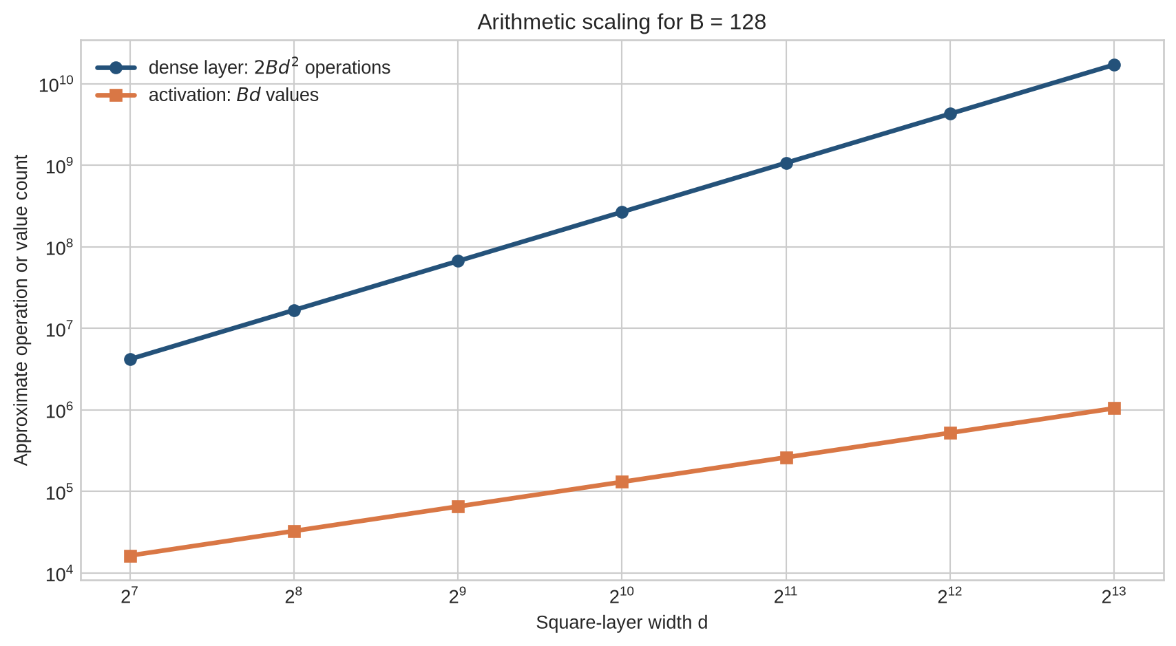
A dense layer performs roughly $2Bd_{\mathrm{in}}d_{\mathrm{out}}$ floating-point operations for a batch, while an elementwise activation performs work proportional to the number of output values, $Bd_{\mathrm{out}}$. Matrix multiplication normally dominates arithmetic. The activation still reads and writes the full activation tensor. On accelerators, this can make an unfused activation limited by memory movement rather than arithmetic.
```{python}
#| label: fig-activation-systems
#| fig-cap: "Activation arithmetic grows with output size, while a dense layer's arithmetic also grows with input width."
#| fig-alt: "A log-scale comparison shows approximate dense-layer operations and elementwise activation evaluations as hidden width increases for a fixed batch of 128."
widths = np.array([128, 256, 512, 1024, 2048, 4096, 8192])
batch = 128
dense_ops = 2 * batch * widths**2
activation_evals = batch * widths

fig, ax = plt.subplots(figsize=(9, 5))
ax.plot(widths, dense_ops, marker="o", color=blue, linewidth=2.5,
        label=r"dense layer: $2Bd^2$ operations")
ax.plot(widths, activation_evals, marker="s", color=orange, linewidth=2.5,
        label=r"activation: $Bd$ values")
ax.set_xscale("log", base=2)
ax.set_yscale("log")
ax.set_xlabel("Square-layer width d")
ax.set_ylabel("Approximate operation or value count")
ax.set_title("Arithmetic scaling for B = 128")
ax.legend()
plt.tight_layout()
plt.show()
```
The separation in operation counts should not be read as an equivalent separation in elapsed time. A matrix-multiplication kernel can achieve high device utilisation through data reuse, whereas a separate activation kernel may spend much of its time moving values. Compilers and specialised kernels therefore fuse bias addition, activation, dropout, or related operations when the architecture permits it. Fusion reduces intermediate memory traffic and kernel-launch overhead without changing the mathematical function.
### Backward passes need activation information
ReLU's backward pass needs to know which pre-activations were positive. Smooth functions may need either the input or output to calculate their derivatives efficiently. Training frameworks save such tensors during the forward pass, increasing activation memory. Activation checkpointing saves memory by retaining fewer intermediate values and recomputing them during backpropagation. The trade-off is additional computation.
Lower numerical precision introduces further considerations. Stable sigmoid implementations avoid directly evaluating expressions that overflow for large magnitudes. Approximate GELU formulas replace the Gaussian cumulative distribution function with cheaper expressions. An approximation that is adequate in one precision and hardware stack should still be tested in the intended training and inference configuration.
### A defensible activation choice is an empirical design decision
A systems review should record:
- the activation and its exact parameterisation;
- where it appears, including hidden, gated, and output locations;
- the distribution of pre-activations and the fraction of inactive or saturated units;
- gradient norms across depth;
- compatibility with initialisation, normalisation, and residual connections;
- available fused kernels in the target precision and hardware;
- task quality, training stability, memory use, throughput, and latency under a controlled comparison.
Changing an activation while also changing width, initialisation, normalisation, or optimiser settings does not isolate the activation's effect. The appropriate choice is the one supported by measurements for the complete architecture and deployment setting.
## Common misconceptions
- **A deeper stack is nonlinear by definition.** A stack of affine layers remains affine unless a nonlinear operation intervenes.
- **ReLU removes a neuron permanently whenever its input is negative.** It sets that unit's output to zero for the current observation; other observations may activate it.
- **A zero ReLU output means the corresponding weight is zero.** The weighted sum and bias may simply produce a negative pre-activation.
- **Sigmoid outputs are automatically calibrated probabilities.** Calibration depends on training, data, loss, and evaluation, not only the output range.
- **Tanh never has vanishing gradients because its derivative is one at zero.** Its derivative approaches zero for large positive and negative inputs.
- **ReLU has no saturation problem.** It does not saturate for positive inputs, but its negative side has zero slope.
- **GELU is a smooth ReLU with the same derivative everywhere.** GELU is a distinct function and can have a small negative derivative in part of its domain.
- **Non-differentiability at zero prevents ReLU training.** Automatic-differentiation libraries use a conventional subgradient at that point.
- **The activation with the best benchmark result is best for every network.** Reported comparisons depend on architecture, training procedure, data, and implementation.
- **Elementwise activations have negligible systems cost.** Their arithmetic is small relative to a matrix multiplication, but tensor reads, writes, and kernel launches can remain material.
- **Changing the activation changes only the forward pass.** It also changes local derivatives, saved tensors, gradient flow, and potentially fused kernels.
## Exercises
1. Show that three affine layers can be rewritten as one affine layer. Identify the combined weight and bias.
2. Evaluate ReLU, sigmoid, and tanh at $z=-1$, $0$, and $1$.
3. Apply ReLU to $z=(2,1.5,-1.5)$ and explain each coordinate.
4. With upstream gradient $(0.6,-0.4,1.2)$, calculate the gradient through ReLU for the running example.
5. Derive the three-region formula for $\operatorname{ReLU}(2x+1)-\operatorname{ReLU}(2x-1)$.
6. Identify the active hidden units at $x=-1$, $x=0$, and $x=1$ in the scalar network.
7. Explain why sigmoid's derivative cannot exceed $0.25$.
8. Calculate tanh's derivative at zero and describe what happens as $|z|$ grows.
9. Implement ReLU and its backward pass in NumPy without using `np.maximum`.
10. Compare `torch.relu`, `torch.sigmoid`, `torch.tanh`, and `torch.nn.functional.gelu` over inputs from $-5$ to $5$.
11. Use finite differences to estimate the ReLU derivative at $z=-1$, $z=1$, and $z=0$. Explain the result at zero.
12. Construct a ReLU unit that is inactive for every observation in a small dataset, then change its bias so that at least one observation activates it.
13. Explain why a separate activation kernel can be limited by memory traffic even when its arithmetic cost is small.
14. For $B=128$ and $d=4096$, compare $Bd$ activation values with approximately $2Bd^2$ dense-layer operations.
15. Design a controlled experiment comparing ReLU and GELU. State which settings must remain fixed and which outcomes should be measured.
16. A binary classifier uses a sigmoid output and binary cross-entropy. Explain why replacing the output sigmoid with ReLU changes the output contract, even if ReLU remains appropriate for hidden layers.
## Summary
Affine layers can change dimension, rotate, rescale, and shift values, but any stack containing only affine operations reduces to one affine map. An activation function prevents that collapse by changing each pre-activation before the next layer. ReLU creates input-dependent affine regions; sigmoid and tanh produce bounded smooth transformations; GELU smoothly attenuates inputs according to a Gaussian weighting.
The activation's derivative determines local gradient transmission. Saturating functions can repeatedly shrink gradients, while ReLU passes positive-side gradients and blocks negative-side gradients. These properties interact with initialisation, data, normalisation, depth, and the training procedure.
At system scale, elementwise activations require less arithmetic than dense matrix multiplication but still move full tensors and store information for backpropagation. Kernel fusion, recomputation, numerical approximation, and hardware support therefore form part of activation choice. Architecture-level evidence is more informative than a context-free ranking of scalar functions.
## Looking ahead
Chapters 2–7 have introduced the components of a trainable neural network separately: predictions, loss, parameter updates, backpropagation, neurons, layers, and activations. [Chapter 8](08-small-neural-network.qmd) assembles them into one small network and follows a complete training loop from data to updated predictions.
## Further reading
The approximation result for sigmoidal networks is established by @cybenko1989. Training difficulties associated with sigmoid and tanh saturation are analysed by @glorot2010. Rectified activations are examined by @nair2010 and @glorot2011. GELU is introduced by @hendrycks2016gelu, the activation search that produced Swish is reported by @ramachandran2017, and gated Transformer variants are evaluated by @shazeer2020. The relation between depth and measures of functional complexity is studied by @raghu2017expressive.