---
title: "Next-token Prediction"
subtitle: "Learning conditional distributions over a vocabulary"
---
## The problem
Chapter 24 ended with the interface: text becomes a sequence of vocabulary identifiers. The identifiers alone predict nothing. A language model assigns a conditional probability distribution to the next identifier given a permitted prefix, and that distribution — not a sentence — is the direct output of a decoder model before any generation rule chooses a continuation.
This chapter defines that objective, its cross-entropy loss, and its limits. Training changes parameters so that observed next tokens receive higher probability under the prefixes supplied by the training data, and nothing beyond that: the objective makes no claim about truth, usefulness, or safety. The chapter therefore distinguishes model probabilities from selected output tokens, and teacher-forced training from sequential inference. Chapter 26 examines the data and scale that determine what a base model can learn; Chapter 28 compares practical decoding rules.
### A five-token sequence makes the objective visible
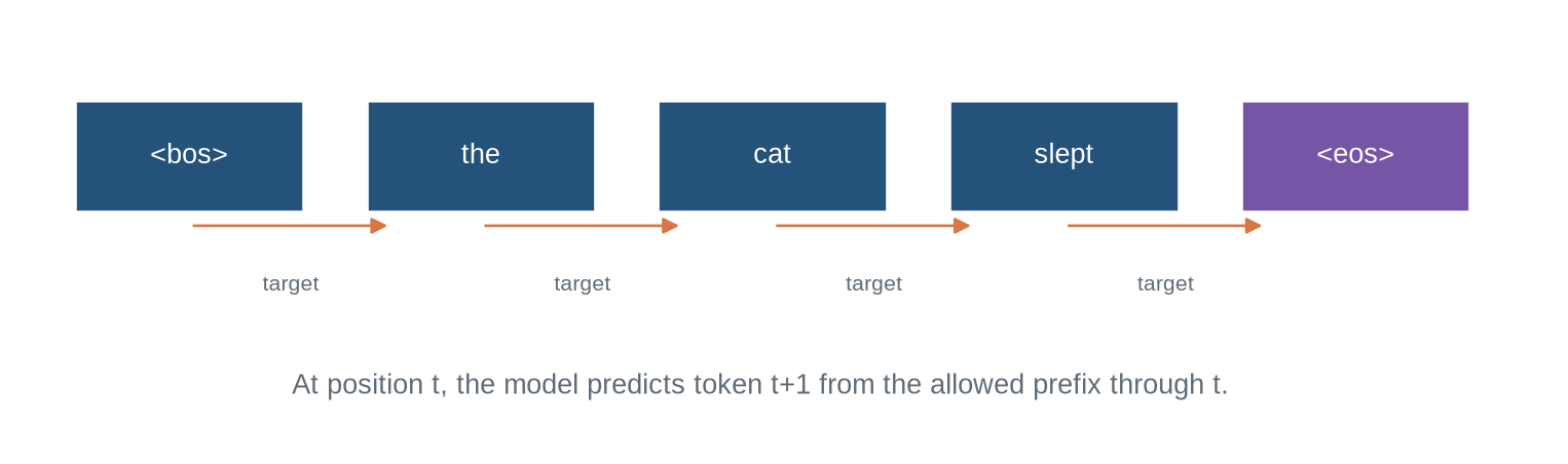
The running sequence is `<bos> the cat slept <eos>`. At each position the model may use only the tokens to its left, and the target for a position is the subsequent token. The whole chapter keeps these five tokens, so every loss, shift, and mask can be checked by hand.
The first diagram shows the training task. Each arrow starts at a prefix position and ends at the token the model must predict from it. Notice that one five-token sequence creates four prediction events: every position contributes its own local training signal.
```{python}
#| label: fig-next-token-task
#| fig-cap: "Next-token training presents a prefix and scores the probability assigned to the following token."
#| fig-alt: "A five-token sequence is shown with arrows from each prefix position to the next target token."
import numpy as np
import matplotlib.pyplot as plt
from matplotlib.patches import Rectangle, FancyArrowPatch
plt.style.use("seaborn-v0_8-whitegrid")
blue,teal,orange,purple,grey="#24527a","#3a9188","#d97745","#7655a6","#5f6b76"
tokens=["<bos>","the","cat","slept","<eos>"]
fig,ax=plt.subplots(figsize=(10,2.8)); ax.axis("off")
for i,t in enumerate(tokens):
    x=.35+i*1.85; ax.add_patch(Rectangle((x,1.15),1.45,.55,facecolor=blue if i<4 else purple,edgecolor="white")); ax.text(x+.725,1.425,t,ha="center",va="center",color="white")
    if i<4: ax.add_patch(FancyArrowPatch((x+.72,1.08),(x+2.02,1.08),arrowstyle="-|>",color=orange,mutation_scale=12)); ax.text(x+1.37,.76,"target",ha="center",color=grey,fontsize=8)
ax.text(4.7,.25,"At position t, the model predicts token t+1 from the allowed prefix through t.",ha="center",color=grey)
ax.set_xlim(0,9.7); ax.set_ylim(0,2.1); plt.show()
```
Every arrow points right, and the model never sees an arrow's endpoint as input at the position where it predicts: at position $t$, only tokens up to $t$ are available. That single rule — predict the next token from a permitted prefix — is the whole objective, and the rest of the chapter formalises it.
::: {.concept-box .concept-core #concept-next-token-prediction data-term="Next-token prediction" data-domain="Large language models"}
**Next-token prediction.** A training objective that estimates a conditional distribution over the next token given an earlier token prefix. It trains a language model's distribution; it does not by itself specify a user task or a decoding policy.
:::
::: {.concept-box .concept-distinction #concept-token-loss-task-outcome data-term="Token loss and task outcome" data-domain="Large language models"}
**Token loss and task outcome.** Token loss measures fit to the next-token target under a specified data distribution. A task outcome measures a separately defined property of a completed system response. Improvement in one does not establish improvement in the other.
:::
## Level 1 - Intuition
### The output is a distribution, not a sentence
After a decoder Transformer processes a prefix, its final representation at the latest usable position is transformed into one score for each vocabulary item. Those scores become probabilities through softmax. A high probability means that, under the model and the supplied prefix, that token is assigned more probability mass than alternatives. It does not mean that the token is true, intended by an author, safe to emit, or the only defensible continuation.
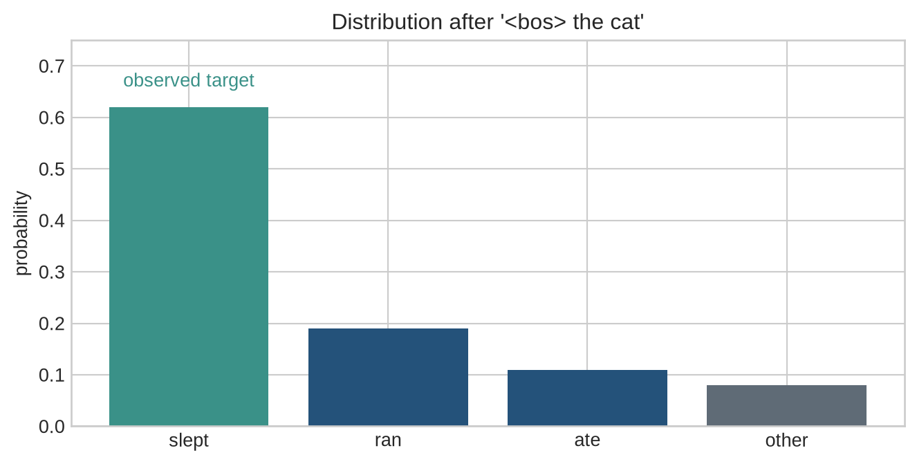
For the prefix `<bos> the cat`, a training example may identify `slept` as the observed next token. The objective rewards the model for assigning it high probability, while assigning probability across every vocabulary entry. The model is not trained from a sentence-level label saying that the complete continuation is good. It receives many local prediction events derived from sequences.
```{python}
#| label: fig-probability-mass
#| fig-cap: "A probability distribution allocates all mass across the vocabulary; the observed target receives a loss determined by its own assigned probability."
#| fig-alt: "A bar chart gives probabilities for slept, ran, ate, and other, with slept marked as the observed target."
names=np.array(["slept","ran","ate","other"]); probs=np.array([.62,.19,.11,.08])
fig,ax=plt.subplots(figsize=(7,3.6)); bars=ax.bar(names,probs,color=[teal,blue,blue,grey]); ax.set_ylim(0,.75); ax.set_ylabel("probability"); ax.set_title("Distribution after '<bos> the cat'")
ax.text(0,.66,"observed target",ha="center",color=teal); plt.tight_layout(); plt.show()
```
The target probability is enough to calculate the loss for this example: `-log(0.62)`. It falls as the model assigns more mass to the observed target and rises sharply when the target probability approaches zero. The remaining probabilities still matter because softmax couples them: increasing one logit changes the normalised distribution.
### Sequence probability is built from conditional probabilities
For token IDs $x_1,\ldots,x_T$, an autoregressive model defines
$$
p(x_1,\ldots,x_T)=\prod_{t=1}^{T}p(x_t\mid x_{<t}).
$$
The notation says that the probability of the whole sequence is decomposed into conditional choices. A beginning marker commonly supplies an initial context. A causal mask, introduced in Chapters 20 and 23, prevents a prediction position from reading later tokens when the model computes all training positions in parallel.
This factorisation does not imply that language is generated word by word. It operates over the token units defined in Chapter 24. One visible word can require several decisions, and an end marker is also a prediction event.
Level 1 identified the prediction events and the distributional output. Level 2 makes the path from logits to loss explicit, including the input-target shift that batches require.
## Level 2 - Mechanics
### Logits become probabilities through softmax
Let $z\in\mathbb{R}^{|V|}$ be the output logits for one position. For vocabulary entry $j$,
$$
p_j=\frac{\exp(z_j)}{\sum_{k=1}^{|V|}\exp(z_k)}.
$$
Logits are unconstrained real numbers; probabilities are non-negative and sum to one. Adding the same constant to every logit does not alter softmax, which permits a stable implementation that subtracts the largest logit before exponentiating.
```{python}
def stable_softmax(logits):
    shifted=logits-np.max(logits)
    weights=np.exp(shifted)
    return weights/weights.sum()

logits=np.array([2.0,0.8,0.2,-0.1])
probabilities=stable_softmax(logits)
print(np.round(probabilities,3), probabilities.sum())
```
The output projection has one column or row per vocabulary item, depending on notation. Vocabulary size therefore affects both the embedding interface and the final prediction interface. A tokenizer mismatch changes what each output index denotes, so an otherwise compatible checkpoint cannot be safely used with a rearranged vocabulary.
### Cross-entropy selects the observed target
For a one-hot target ID $y$, the negative log likelihood is $-\log p_y$. Over valid sequence positions, the usual language-modelling loss averages those values:
$$
\mathcal{L}=-\frac{1}{N}\sum_{n=1}^{N}\log p_\theta(x_n\mid x_{<n}).
$$
Here $N$ must count valid predicted tokens, not padded tensor cells. Cross-entropy is a name for the same calculation when the target distribution is one-hot. It compares a target distribution with the model distribution; it does not assess factuality, instruction-following, or downstream usefulness.
```{python}
target_id=0
loss=-np.log(probabilities[target_id])
print("target probability:",round(probabilities[target_id],3),"loss:",round(loss,3))
```
### Training shifts inputs and targets
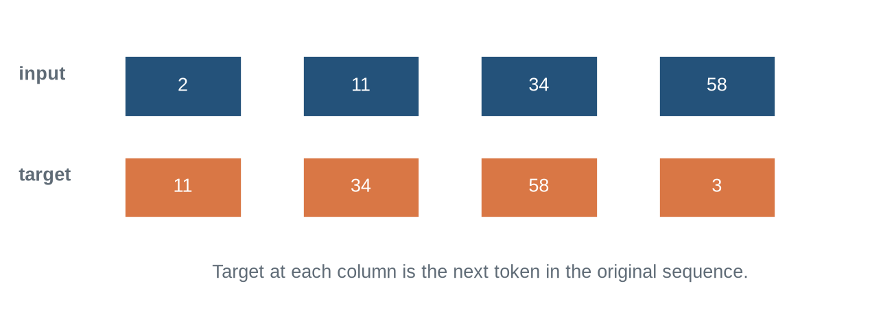
For a stored sequence `[<bos>, the, cat, slept, <eos>]`, the model input may be the first four IDs and targets the final four IDs. Each input position produces a distribution for the token one place to the right. The full prefix is supplied to compute those positions efficiently, but the causal mask preserves the conditional information boundary.
```{python}
sequence=np.array([2,11,34,58,3])
inputs,targets=sequence[:-1],sequence[1:]
print("inputs: ",inputs)
print("targets:",targets)
```
An off-by-one error can make the model predict the current input token, expose the next target as input, or omit the end marker. These errors can produce plausible shapes and falling losses, so exact small examples should be inspected before a large run.
```{python}
#| label: fig-shifted-targets
#| fig-cap: "Teacher-forced language-model batches align each input position with the following target ID."
#| fig-alt: "Two aligned rows show input IDs 2, 11, 34, 58 above target IDs 11, 34, 58, 3, with arrows indicating the one-position shift."
fig,ax=plt.subplots(figsize=(8.5,2.8)); ax.axis("off")
for row,(label,values,colour) in enumerate([("input",inputs,blue),("target",targets,orange)]):
    ax.text(.05,1.72-row*.8,label,weight="bold",color=grey)
    for i,v in enumerate(values):
        x=1+i*1.6; ax.add_patch(Rectangle((x,1.43-row*.8),1.05,.48,facecolor=colour,edgecolor="white")); ax.text(x+.525,1.67-row*.8,str(v),ha="center",va="center",color="white")
ax.text(4.2,.15,"Target at each column is the next token in the original sequence.",ha="center",color=grey); ax.set_xlim(0,7.8); ax.set_ylim(0,2.25); plt.show()
```
Level 2 specified softmax, the masked loss average, and the target shift. Level 3 connects those pieces to the decoder's representations and output head, and tests the resulting contracts in code.
## Level 3 - Mathematics & Code
### Causal representations and the output head
Let $h_t\in\mathbb{R}^{d}$ be the decoder representation at position $t$, computed with causal access to $x_{\leq t}$. An output head produces $z_t=W h_t+b$, where $W$ has a vocabulary axis. Softmax turns $z_t$ into $p_\theta(\cdot\mid x_{\leq t})$. Depending on the indexing convention, this distribution is trained against $x_{t+1}$. Weight tying can use the input embedding matrix in the output projection, but it does not remove the vocabulary distribution or change the target shift.
```{python}
hidden=np.array([.4,-.2,.6])
W=np.array([[.2,.1,-.3],[-.4,.5,.2],[.1,-.2,.7],[.3,.3,.1]])
b=np.array([.0,.1,-.1,.0])
logits=W@hidden+b
print("logits:",np.round(logits,3))
print("probabilities:",np.round(stable_softmax(logits),3))
```
### Masks determine which losses count
In a padded batch, valid-token masks usually govern both attention eligibility and loss aggregation, but they are not interchangeable with causal masks. The causal mask forbids future access. The valid-token mask removes artificial positions. An implementation must specify whether it predicts an end token, whether packed documents permit cross-document attention, and whether loss includes special markers.
```{python}
logit_batch=np.array([[[2.,.5],[.1,1.3]],[[.7,.2],[1.1,.4]]])
target_batch=np.array([[0,1],[0,0]])
valid=np.array([[1,1],[1,0]],dtype=bool)
token_losses=np.array([-np.log(stable_softmax(row)[target]) for rows,targets in zip(logit_batch,target_batch) for row,target in zip(rows,targets)]).reshape(2,2)
masked_loss=(token_losses*valid).sum()/valid.sum()
print(np.round(token_losses,3)); print("masked mean:",round(masked_loss,3))
```
The example has deliberately separate names for the tensor and mask axes. A loss averaged over all four cells would silently reward or penalise a padding placeholder. The equivalent issue arises when an incorrect attention mask lets padding or a later target affect a valid prediction.
### Perplexity is a transformed loss, not a general evaluation
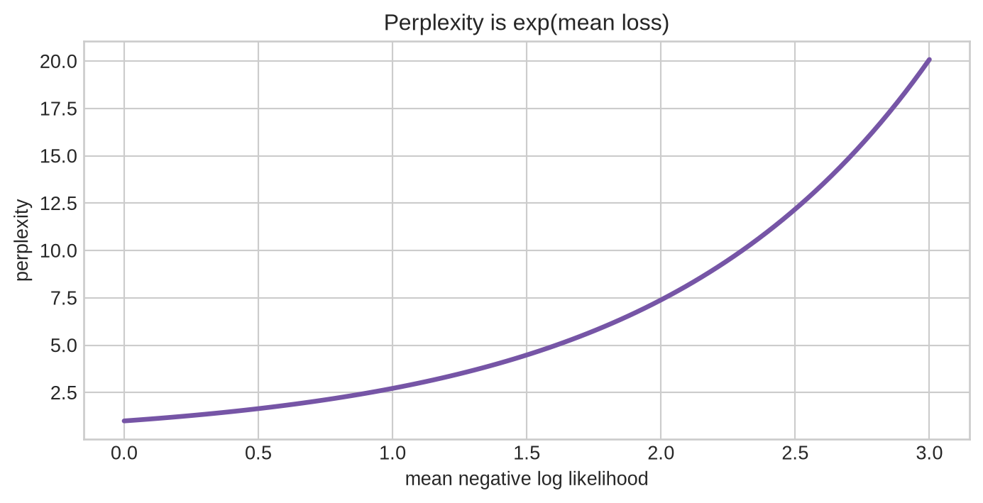
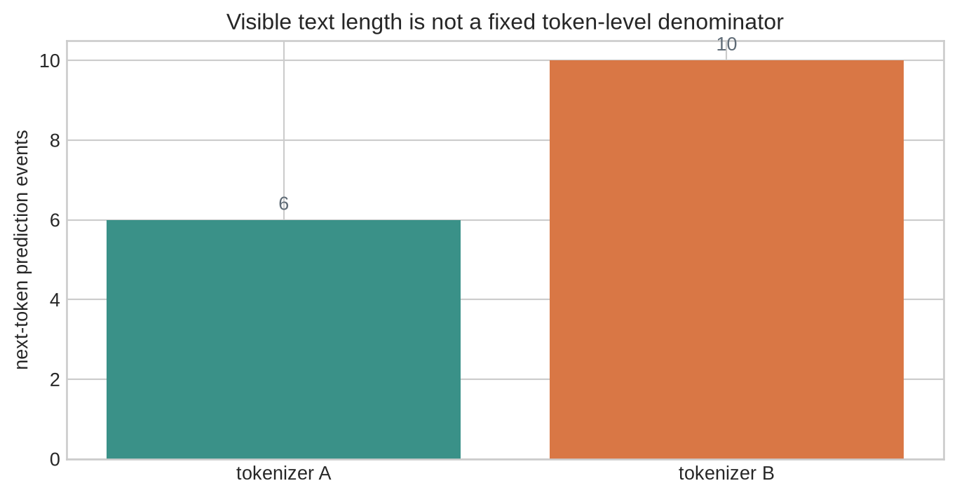
Perplexity is commonly $\exp(\mathcal{L})$ when the loss uses natural logarithms. It can be interpreted as an effective branching factor under the particular tokenisation and evaluation corpus. Comparing perplexity across different tokenizers is generally invalid because one model may make more prediction events per visible string. It also does not measure whether continuations are accurate for a user task, calibrated under distribution shift, or appropriate after decoding.
```{python}
mean_nll=np.array([.69,1.39,2.30])
print("losses:",mean_nll)
print("perplexities:",np.round(np.exp(mean_nll),2))
```
```{python}
#| label: fig-loss-perplexity
#| fig-cap: "Perplexity rises exponentially with average negative log likelihood, so equal changes in loss do not produce equal changes in perplexity."
#| fig-alt: "A curve plots perplexity against average negative log likelihood from zero to three."
loss_grid=np.linspace(0,3,100)
fig,ax=plt.subplots(figsize=(7.3,3.8)); ax.plot(loss_grid,np.exp(loss_grid),color=purple,lw=2.5); ax.set_xlabel("mean negative log likelihood"); ax.set_ylabel("perplexity"); ax.set_title("Perplexity is exp(mean loss)"); plt.tight_layout(); plt.show()
```
Level 3 implemented the output head, the masked loss, and the perplexity transform. Level 4 audits what the objective estimates and what it leaves open: the training-inference difference, the boundaries of evaluation units, and the context conventions a reported loss depends on.
## Level 4 - Research & Systems
### Training and generation have different inputs
Teacher forcing supplies observed previous tokens at every training position. At inference, the model receives its own selected token from the preceding step. This difference is operational rather than a contradiction in the objective: the same conditional distribution is evaluated repeatedly, but the prefix source changes. A single wrong early selection can therefore move a generation into a prefix region poorly represented in training data.
```{python}
prefix=[2]
chosen=[11,34,58,3]
for token in chosen:
    # In a real model, probabilities depend on the current prefix.
    print("prefix",prefix,"-> choose",token)
    prefix.append(token)
```
The objective identifies a probability distribution. A decoding rule chooses from it. Greedy decoding selects the highest-probability token; sampling draws according to some transformed distribution; constrained systems may reject choices or stop at defined markers. Treating an argmax token as the model's only belief discards the distribution that training actually produced.
```{python}
np.random.seed(4)
print("greedy ID:",int(probabilities.argmax()))
print("sampled IDs:",np.random.choice(len(probabilities),size=8,p=probabilities))
```
### A minimal audit
An objective audit should record the tokenizer and vocabulary version, position convention, input-target shift, output-head shape, causal-mask orientation, padding convention, loss denominator, document-boundary policy, special-token treatment, precision used for softmax and loss, and the metric corpus. A checkpoint cannot be interpreted from its parameter count alone.
Tests should include a hand-calculated one-position loss, invariance of an earlier prediction to a changed future token, invariance to additional padding, and agreement between the batch loss and the mean of valid token losses. They should also check that generation begins from the intended start context and that an end marker stops only under the declared generation policy.
```{python}
assert np.isclose(stable_softmax(logits).sum(),1.0)
assert inputs.shape==targets.shape
assert valid.sum()==3
assert np.isfinite(masked_loss)
print("basic objective-interface checks passed")
```
### What the likelihood objective estimates
The loss is evaluated on tokens observed in a corpus. It estimates how well the model distribution matches the evaluation distribution under the chosen representation and context rule. A low average loss on a held-out sample is evidence about that predictive task. It is not evidence that the sample is representative of all future use, that the corpus is accurate, or that a continuation selected at inference will satisfy a different quality criterion.
This distinction is practical. The corpus can contain duplicated text, inconsistent claims, private conventions, or sequences that are unsuitable as answers. A model that assigns those sequences probability has learned a regularity of its training distribution. Whether that regularity should be surfaced in an application depends on the training data, adaptation procedure, system instructions, retrieval context, and decoding rule. Later chapters address those additional components; they should not be attributed to the next-token loss alone.
The objective also makes no independent decision about the unit of evaluation. The same visible sentence can have different losses under different tokenizers because it contains different numbers of prediction events. A report should therefore state the tokenizer, maximum context length, preprocessing, split construction, whether document boundaries are preserved, and whether the reported loss includes special markers. Without those details, a perplexity comparison can describe different quantities under the same label.
```{python}
#| label: fig-tokenisation-metric
#| fig-cap: "The same visible text can create different numbers of prediction events under different tokenisations, making raw perplexity comparisons across tokenizers inappropriate."
#| fig-alt: "A conceptual bar chart compares two tokenizers that represent one sentence with six and ten prediction events."
fig,ax=plt.subplots(figsize=(7.2,3.8))
ax.bar(["tokenizer A","tokenizer B"],[6,10],color=[teal,orange])
ax.set_ylabel("next-token prediction events")
ax.set_title("Visible text length is not a fixed token-level denominator")
for i,n in enumerate([6,10]): ax.text(i,n+.25,str(n),ha="center",color=grey)
plt.tight_layout(); plt.show()
```
### Context boundaries are part of the example definition
The conditional notation hides an operational choice: which earlier tokens count as the prefix. In a document-level corpus, a beginning marker or separator may indicate that one text has ended and another has begun. If preprocessing concatenates documents without a boundary policy, the model can be trained to predict the start of one item from the end of an unrelated item. Packing can improve hardware utilisation, but its attention and loss masks must state whether tokens may attend across packed segments.
Finite context windows create a second boundary. A position near the end of a long sequence is conditioned on the retained window, not necessarily the entire preceding document. The objective is still a conditional likelihood, but the condition is truncated. This affects claims about long-range dependence and makes maximum length a property of the trained system rather than a deployment-only setting. Chapter 27 examines the inference and systems consequences of finite context in detail.
```{python}
document=np.array([2,11,34,58,71,89,3])
window=4
for end in range(1,len(document)):
    start=max(0,end-window)
    print("context",document[start:end],"target",document[end])
```
### Error analysis starts with the conditional event
An average loss can conceal very different patterns. A model may perform well on frequent punctuation and common short tokens while assigning poor probability to dates, names, a language variety, or a rare formatting sequence. Error analysis should therefore retain token-level events and group them by a declared property: position in the document, token frequency, script, source, length, or task-relevant category. Such groups are descriptive only when their construction and sample sizes are reported.
The most probable alternative is often informative, but it should not be treated as a diagnosis by itself. If the target `slept` receives little probability after a clear prefix, the distribution may prefer a semantically related verb, a frequent generic continuation, or a tokenisation-dependent fragment. Inspecting the prefix, target, alternative tokens, and preprocessing records makes the failure analysable. A generated continuation alone does not reveal whether the error began in the model distribution, a decoding decision, or an input-interface mismatch.
```{python}
vocab=np.array(["slept","ran","ate","<eos>"])
rank=np.argsort(probabilities)[::-1]
for idx in rank:
    print(vocab[idx],round(probabilities[idx],3))
```
## Common misconceptions
- **The largest logit is already a probability.** Logits become probabilities only after normalisation.
- **A low loss proves a model is truthful.** Loss rewards agreement with held-out token sequences under a specified distribution.
- **Teacher forcing means the model sees future targets.** It supplies earlier observed tokens; a causal mask must still block later positions.
- **Perplexity can compare any two language models.** Tokenisation, corpus, preprocessing, and loss conventions must match.
- **Next-token prediction specifies how a model should answer a person.** It defines a base predictive objective; adaptation and decoding remain separate choices.
- **Padding is harmless without an explicit mask.** It can affect attention and loss unless the implementation excludes it.
## Exercises
1. Write the conditional factorisation for a four-token sequence.
2. Compute softmax probabilities for logits `[0, 0]`.
3. Calculate the negative log likelihood when the target probability is 0.2.
4. Explain why adding 100 to every logit leaves softmax unchanged.
5. Shift a six-token sequence into language-model inputs and targets.
6. Identify the loss denominator for a padded batch with valid lengths 3 and 5.
7. Draw a causal attention eligibility matrix for four positions.
8. Implement a numerically stable log-softmax.
9. Show with a test that a changed future token cannot change an earlier causal output.
10. Explain why a vocabulary permutation requires a matching output-head permutation.
11. Compare token-level and character-level perplexity reporting.
12. State whether end-of-sequence prediction is included in a given objective and why.
13. Construct an example in which greedy decoding and sampling select different next tokens.
14. List metadata required to reproduce a reported validation loss.
15. Explain how teacher forcing and autoregressive inference create different prefixes.
16. State which later chapter compares practical decoding policies.
## Summary
Next-token prediction trains a causal language model to assign probability to the observed subsequent token under an allowed prefix. Logits are normalised by softmax, and cross-entropy averages the negative log probability of valid targets. The target shift, causal mask, padding policy, vocabulary mapping, and loss denominator are part of the objective definition.
The training objective produces conditional distributions, not directly a finished answer or a factual guarantee. Generation applies a selection rule sequentially to those distributions. [Chapter 26](26-pretraining-data-objectives-scale.qmd) examines the data, objectives, and scale that shape a base model before Chapter 28 treats decoding rules in detail.
## Looking ahead
Next-token prediction specifies the objective applied to a token sequence. [Chapter 26](26-pretraining-data-objectives-scale.qmd) examines how the training corpus, data-processing rules, token budget, and scale choices determine what that objective is actually fitted to.
## Further reading
The neural probabilistic language model is set out by @bengio2003neural. The Transformer decoder objective and causal masking convention are specified by @vaswani2017.