---
title: "Tokens and Tokenisation"
subtitle: "Turning text into the discrete identifiers a model can process"
---
## The problem
Chapter 23 compared Transformer families as arrangements of information flow, but every one of them consumes the same kind of input: a sequence of discrete identifiers drawn from a fixed vocabulary. Raw text is not that. A Transformer processes tensors, not character strings, and before any embedding lookup something must decide which pieces of text count as units and which integers represent them.
That decision is tokenisation, and it is part of the model rather than a harmless pre-processing detail. It determines which distinctions the model can represent directly, the sequence length it receives, the cost of attention, and whether training, evaluation, and inference inputs are compatible with one another. This chapter defines the text-to-ID contract, compares word, character, byte, and subword units, and explains how vocabulary and normalisation choices affect coverage and cost. It does not yet define the probability distribution or training loss over the resulting IDs; Chapter 25 does that.
### A repeated word makes segmentation visible
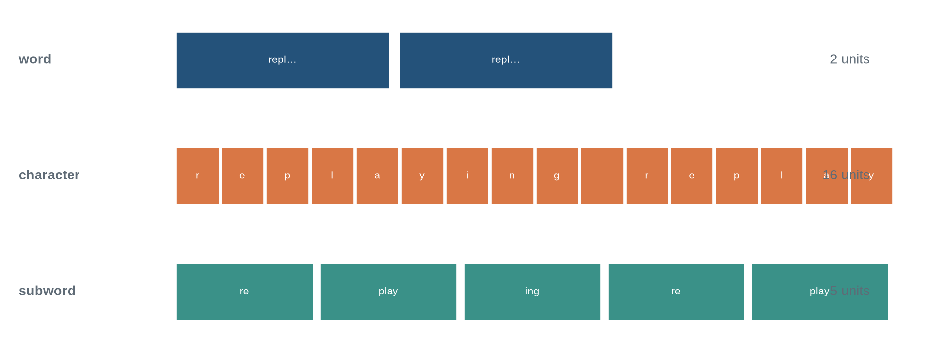
The running text is `replaying replay`. The repeated form makes it possible to compare a word-level representation, a character sequence, and a subword segmentation without implying that any one segmentation is intrinsically correct.
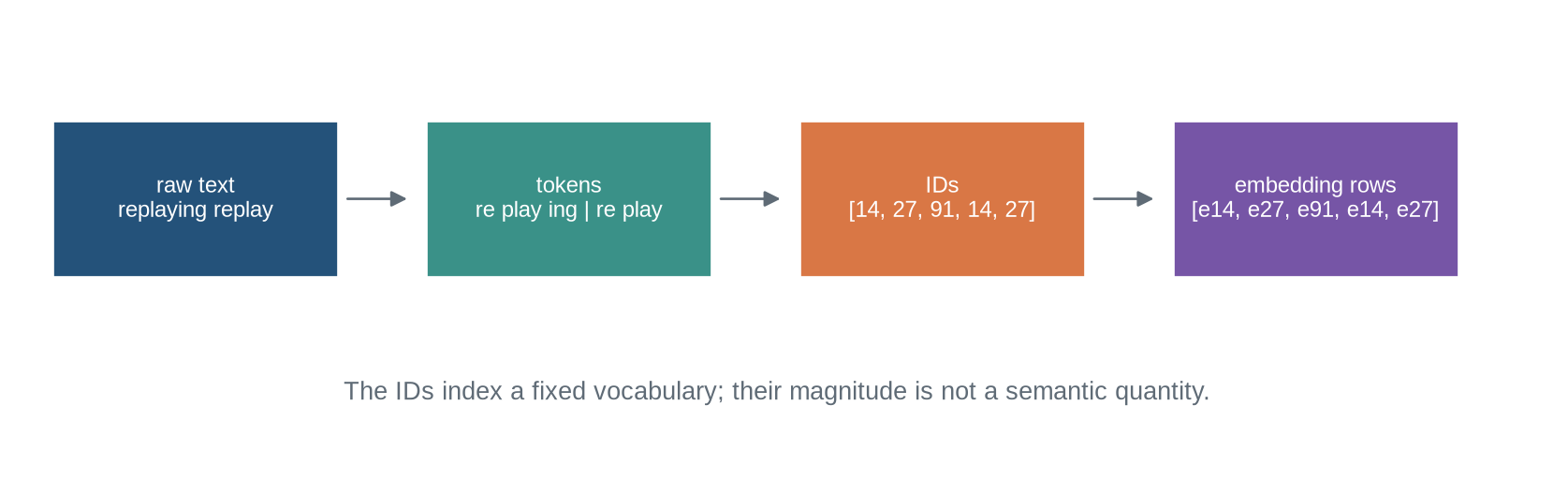
The first diagram follows the whole interface from left to right: raw text becomes token strings, token strings become integer IDs, and IDs select embedding rows. Notice where meaning does and does not enter — the IDs are addresses into a fixed vocabulary, and their magnitudes are not semantic quantities.
```{python}
#| label: fig-text-to-ids
#| fig-cap: "Tokenisation maps text to token strings and then to vocabulary identifiers; embedding lookup later maps those identifiers to learned vectors."
#| fig-alt: "A left-to-right diagram shows raw text, subword pieces, integer token IDs, and corresponding embedding vectors."
import numpy as np
import matplotlib.pyplot as plt
from matplotlib.patches import Rectangle, FancyArrowPatch

plt.style.use("seaborn-v0_8-whitegrid")
blue,teal,orange,purple,grey="#24527a","#3a9188","#d97745","#7655a6","#5f6b76"
fig,ax=plt.subplots(figsize=(11,3.2)); ax.axis("off")
items=[("raw text\nreplaying replay",blue),("tokens\nre play ing | re play",teal),("IDs\n[14, 27, 91, 14, 27]",orange),("embedding rows\n[e14, e27, e91, e14, e27]",purple)]
for i,(label,colour) in enumerate(items):
    x=.25+i*2.68; ax.add_patch(Rectangle((x,1.05),2.05,.72,facecolor=colour,edgecolor="white")); ax.text(x+1.025,1.41,label,ha="center",va="center",color="white",fontsize=9)
    if i<3: ax.add_patch(FancyArrowPatch((x+2.08,1.41),(x+2.58,1.41),arrowstyle="-|>",mutation_scale=13,color=grey))
ax.text(5.45,.48,"The IDs index a fixed vocabulary; their magnitude is not a semantic quantity.",ha="center",color=grey)
ax.set_xlim(0,11); ax.set_ylim(.2,2.25); plt.show()
```
The right-hand stage belongs to Chapter 17: each ID selects one row of an embedding table. The tokenisation decision is everything to its left — which strings exist as units, how many of them a text needs, and which distinctions survive the conversion.
::: {.concept-box .concept-core #concept-tokenisation data-term="Token and tokenisation" data-domain="Large language models"}
**Token and tokenisation.** A token is a discrete identifier from a model vocabulary. Tokenisation maps text into such identifiers and back again. It changes sequence length, loss units, and which distinctions a language model can directly represent.
:::
## Level 1 - Intuition
### Text must cross a discrete interface
The string `replaying replay` is a sequence of characters visible to a reader. A model needs a finite set of discrete symbols that can index rows in an embedding table. A tokenizer chooses a segmentation, assigns each chosen token a vocabulary ID, and records conventions for spaces, punctuation, Unicode, and special markers. The embedding layer in Chapter 17 then replaces each ID with a learned vector.
An ID is an address, not an ordered quantity. ID 27 is not twice as meaningful as ID 14, and neighbouring IDs do not imply similar tokens. Permuting the rows of an embedding table and applying the same permutation to token IDs leaves the model function unchanged. Meaning is learned in the embedding vectors and later transformations, not in the integers used to retrieve them.
### A token is a modelling unit, not necessarily a word
Word tokenisation gives a readable segmentation but needs a policy for rare or unseen words. Character tokenisation has a small vocabulary and can represent any sequence of known characters, but it creates long sequences. Byte tokenisation can represent arbitrary byte strings under a fixed alphabet, but its pieces may split one human character across several bytes. Subword tokenisation chooses reusable pieces between characters and words.
```{python}
#| label: fig-segmentation-granularity
#| fig-cap: "The same text can be represented as words, characters, or subwords; the choice changes vocabulary coverage and sequence length."
#| fig-alt: "Three labelled rows segment the text replaying replay into two word tokens, sixteen character-like tokens including a space, and five subword tokens."
forms=[("word",["replaying","replay"]),("character",list("replaying replay")),("subword",["re","play","ing","re","play"])]
fig,axes=plt.subplots(3,1,figsize=(10,3.8))
for ax,(name,pieces) in zip(axes,forms):
    ax.axis("off"); ax.text(.01,.5,name,ha="left",va="center",weight="bold",color=grey,transform=ax.transAxes)
    width=min(.74/max(len(pieces),1),.23)
    for i,piece in enumerate(pieces):
        x=.18+i*width*1.05; ax.add_patch(Rectangle((x,.22),width,.56,facecolor=[blue,orange,teal][["word","character","subword"].index(name)],edgecolor="white")); ax.text(x+width/2,.5,piece if len(piece)<5 else piece[:4]+"…",ha="center",va="center",color="white",fontsize=8)
    ax.text(.93,.5,f"{len(pieces)} units",ha="right",va="center",color=grey,transform=ax.transAxes)
plt.tight_layout(); plt.show()
```
No segmentation removes ambiguity from language. Tokenisation determines the discrete units supplied to the model; contextual layers can later combine their representations. A word split that appears linguistically familiar is not automatically superior for prediction, and a subword split need not correspond to a morphological boundary.
Byte-level methods make a different guarantee. A byte vocabulary can represent any input expressed in the chosen byte encoding without requiring an unknown-word token, but a visible character may become several byte tokens. This can be useful for arbitrary strings, mixed scripts, code, or malformed text, while increasing token counts for some inputs. The guarantee concerns representability of bytes; it does not guarantee that a trained model has useful evidence for every resulting sequence.
### Vocabulary coverage has a cost
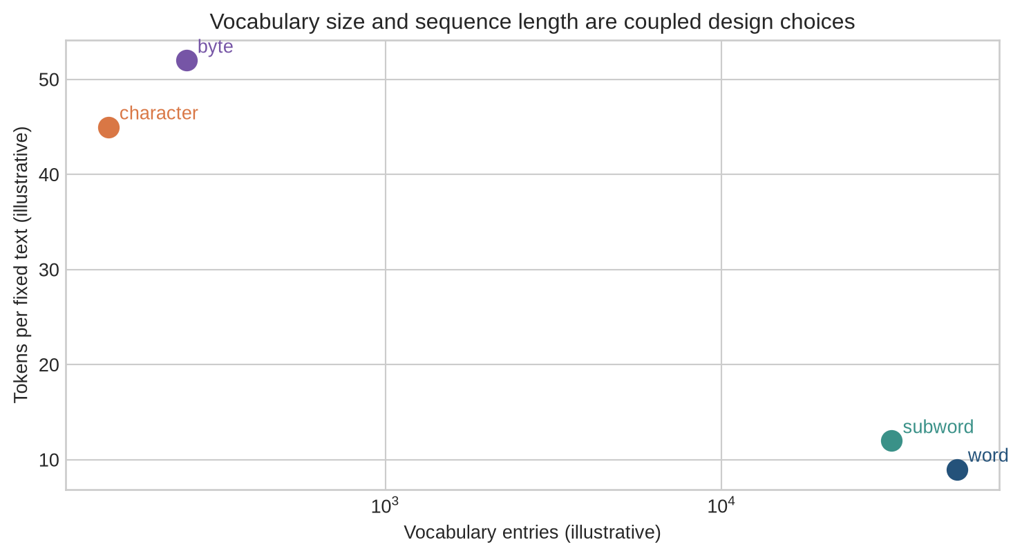
A larger vocabulary can store more frequent whole units and may shorten sequences. It also enlarges the embedding table and the output interface used in token prediction. A smaller vocabulary reduces those tables but usually makes sequences longer. For a Transformer, longer sequences affect attention relations quadratically, as Chapter 20 showed.
The relevant comparison is not simply “fewer tokens is better”. Coverage, language mix, spelling variation, throughput, memory, the training corpus, and the intended task all matter. A tokenizer is fitted or configured on a particular text distribution, then becomes fixed at the model boundary.
```{python}
#| label: fig-vocabulary-length-tradeoff
#| fig-cap: "Vocabulary choices exchange embedding-table size against the average number of tokens needed to represent text; neither axis alone identifies the best tokenizer."
#| fig-alt: "A conceptual scatter plot places word, subword, character, and byte tokenizers at different combinations of vocabulary size and average sequence length."
names=["word","subword","character","byte"]
vocab_sizes=np.array([50000,32000,150,256]); average_lengths=np.array([9,12,45,52])
fig,ax=plt.subplots(figsize=(7.8,4.3))
for name,vocab,length,colour in zip(names,vocab_sizes,average_lengths,[blue,teal,orange,purple]):
    ax.scatter(vocab,length,s=115,color=colour); ax.text(vocab*1.08,length+.8,name,color=colour)
ax.set_xscale("log"); ax.set_xlabel("Vocabulary entries (illustrative)"); ax.set_ylabel("Tokens per fixed text (illustrative)"); ax.set_title("Vocabulary size and sequence length are coupled design choices")
plt.tight_layout(); plt.show()
```
The coordinates are illustrative rather than a benchmark. Actual token counts depend on language, corpus, normalisation, and the particular vocabulary. The point is architectural: a vocabulary entry consumes embedding and output-interface capacity, while a longer segmentation consumes positions and attention relations.
Level 1 established the interface. Level 2 follows its operational steps and failure modes.
## Level 2 - Mechanics
### The tokenizer contract has several stages
A practical pipeline commonly: reads a Unicode string; applies a specified normalisation or preservation policy; inserts or recognises special markers; segments text into token strings; maps strings to IDs; pads, truncates, or packs sequences; and supplies an attention mask alongside IDs. Each stage can change the sequence supplied to the model.
For example, lowercasing can merge distinctions between `May` and `may`. Normalising a Unicode form can make visually similar text share a representation, but it can also erase distinctions relevant to a language or task. A tokenizer must therefore document its transformations rather than treating them as universally neutral cleanup.
```{python}
vocabulary={"<pad>":0,"<unk>":1,"<bos>":2,"<eos>":3,"re":4,"play":5,"ing":6," ":7}
inverse={idx:token for token,idx in vocabulary.items()}
pieces=["<bos>","re","play","ing"," ","re","play","<eos>"]
ids=[vocabulary.get(piece,vocabulary["<unk>"]) for piece in pieces]
print("pieces:",pieces)
print("ids:",ids)
print("decoded pieces:",[inverse[i] for i in ids])
```
The special IDs are ordinary vocabulary entries with an agreed role. They are not self-describing to a model. If one checkpoint treats ID 0 as padding and another treats it as a visible token, their input interfaces are incompatible even when their embedding matrices have the same shape.
The interface also needs a decoding rule. A reversible tokenisation can reconstruct the stored text representation from valid token pieces, but it cannot necessarily recover distinctions already removed by normalisation, lowercasing, truncation, or an unknown-token replacement. “Detokenises correctly” should therefore mean correct under a declared text representation and special-token policy.
### Unknown items, padding, and truncation are distinct policies
An unknown-token policy replaces an unrecognised unit with an available placeholder ID. Padding adds artificial positions so a batch has a common tensor shape. Truncation drops selected positions to meet a maximum length. These operations have different consequences and require different metadata.
Padding should be paired with a padding mask so attention and losses can ignore artificial positions. Truncation can remove content and change a task's answer. An unknown token keeps sequence length but collapses different unseen strings onto one identifier. These are modelling choices that must be tested on the intended distribution.
```{python}
batch_ids=np.array([[2,4,5,6,3,0,0],[2,4,5,7,4,5,3]])
pad_id=0; attention_mask=batch_ids!=pad_id
print("token IDs:\n",batch_ids)
print("valid-token mask:\n",attention_mask.astype(int))
print("valid lengths:",attention_mask.sum(axis=1))
```
The mask uses `True` for valid positions in this example. Frameworks vary in whether an argument expects a valid-token mask or a padding mask, so a model interface must state the convention and include a small test that padded content cannot influence valid outputs.
### Subword vocabularies reuse frequent pieces
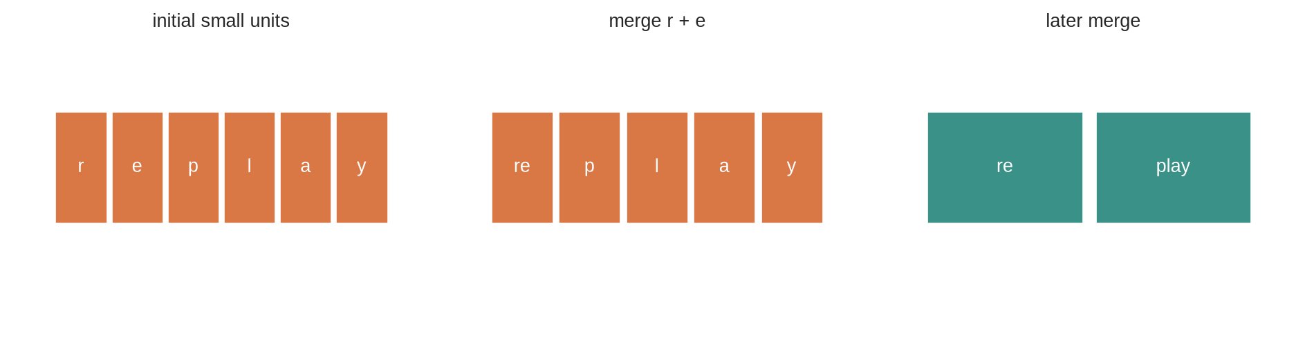
Byte-pair encoding (BPE) begins from small units and repeatedly merges frequent adjacent pairs in a training corpus. The learned merge list defines a vocabulary and a segmentation procedure. Sennrich, Haddow, and Birch used subword units based on BPE to address rare and unknown words in neural machine translation [@sennrich2016bpe].
Unigram-style tokenizers begin with a candidate inventory and select segmentations under a probabilistic vocabulary model. SentencePiece provides BPE and unigram approaches trained directly from raw sentences, avoiding a required language-specific pre-tokenisation stage [@kudo2018sentencepiece]. The algorithms differ, but both make the vocabulary and segmentation rules part of the trained model interface.
```{python}
#| label: fig-bpe-merge
#| fig-cap: "A toy BPE-style merge replaces a frequent adjacent pair with one new piece; repeated merges define the available subword vocabulary."
#| fig-alt: "The token sequence r e p l a y is shown becoming re p l a y after merging r and e, then re play after further merges."
stages=[list("replay"),["re","p","l","a","y"],["re","play"]]
fig,axes=plt.subplots(1,3,figsize=(10,2.7))
for ax,pieces,title in zip(axes,stages,["initial small units","merge r + e","later merge"]):
    ax.axis("off"); ax.set_title(title,fontsize=10); width=.75/max(len(pieces),1)
    for i,piece in enumerate(pieces):
        x=.1+i*width*1.08; ax.add_patch(Rectangle((x,.37),width,.38,facecolor=[blue,teal,orange][min(len(pieces)-1,2)],edgecolor="white")); ax.text(x+width/2,.56,piece,ha="center",va="center",color="white")
plt.tight_layout(); plt.show()
```
The figure is a toy procedure, not a tokenizer trainer. Real BPE implementations define initial symbols, pre-tokenisation or raw-text handling, merge order, vocabulary limits, special tokens, and byte or Unicode representation. These choices affect which strings can be represented and how many IDs they consume.
Segmentation can also be ambiguous. With pieces `re`, `play`, `ing`, and `replay`, the text `replaying` could be divided as `replay` plus `ing` or as `re` plus `play` plus `ing`. A deterministic BPE implementation resolves the choice using its learned merge order; a unigram formulation can score alternatives. The resulting model sees only the selected sequence unless training deliberately samples alternatives. Tokenisation is therefore a learned or configured view of text, not a transparent transcription.
Level 2 followed the stages of the tokenisation contract and their failure modes. Level 3 states the lookup interface formally, implements a small encoder, and counts what tokenisation costs in tensors and attention relations.
## Level 3 - Mathematics & Code
### IDs select rows; they are not numerical features
Let a vocabulary contain $V$ entries and let its embedding matrix be $E\in\mathbb{R}^{V\times D}$. For ID $i_t\in\{0,\ldots,V-1\}$ at position $t$, embedding lookup returns
$$x_t=E_{i_t,:}.$$
For a batch of IDs $I\in\mathbb{N}^{B\times S}$, lookup produces $X\in\mathbb{R}^{B\times S\times D}$. This is the interface between tokenisation and the embeddings in Chapter 17. Replacing an input token changes the selected row; adding one to an ID does not make a meaningful incremental change.
```{python}
import torch
from torch import nn

torch.manual_seed(24)
embedding=nn.Embedding(num_embeddings=len(vocabulary),embedding_dim=4,padding_idx=0)
ids_tensor=torch.tensor(batch_ids)
vectors=embedding(ids_tensor)
print("IDs:",tuple(ids_tensor.shape),"embedding output:",tuple(vectors.shape))
print("same ID gives the same row before contextual layers:",torch.allclose(vectors[0,1],vectors[1,1]))
print("padding row is zeroed by this embedding configuration:",vectors[0,5].detach().numpy().round(4))
```
The equality check uses the same token ID in two positions. Later contextual layers can transform those positions into different representations, but the lookup itself is a row selection. `padding_idx=0` is an implementation policy; it does not remove the need for masks in attention and loss calculations.
### A simple longest-match encoder makes the vocabulary dependence visible
```{python}
def longest_match_encode(text,pieces,unk="<unk>"):
    output=[]; cursor=0; choices=sorted(pieces,key=len,reverse=True)
    while cursor<len(text):
        match=next((piece for piece in choices if text.startswith(piece,cursor)),None)
        if match is None: output.append(unk); cursor+=1
        else: output.append(match); cursor+=len(match)
    return output

piece_inventory={"re","play","ing"," ","<bos>","<eos>"}
print(longest_match_encode("replaying replay",piece_inventory))
print(longest_match_encode("replayed",piece_inventory))
```
The second result contains an unknown item because the toy inventory lacks pieces needed for the final characters. Real systems avoid this particular failure in different ways, including character or byte fallback. The example shows the contract: a segmentation algorithm and an inventory jointly determine what token sequence is available to the model.
```{python}
text="café"
characters=list(text); utf8_bytes=list(text.encode("utf-8"))
print("characters:",characters,"count:",len(characters))
print("UTF-8 byte values:",utf8_bytes,"count:",len(utf8_bytes))
```
The displayed text has four Unicode characters but five UTF-8 bytes because the final character uses more than one byte in that encoding. A byte-level tokenizer works with the latter sequence, while a character-level account works with the former. Neither representation is automatically wrong; they expose different units and different length conventions that should not be mixed in reporting.
### Token counts affect tensor and attention sizes
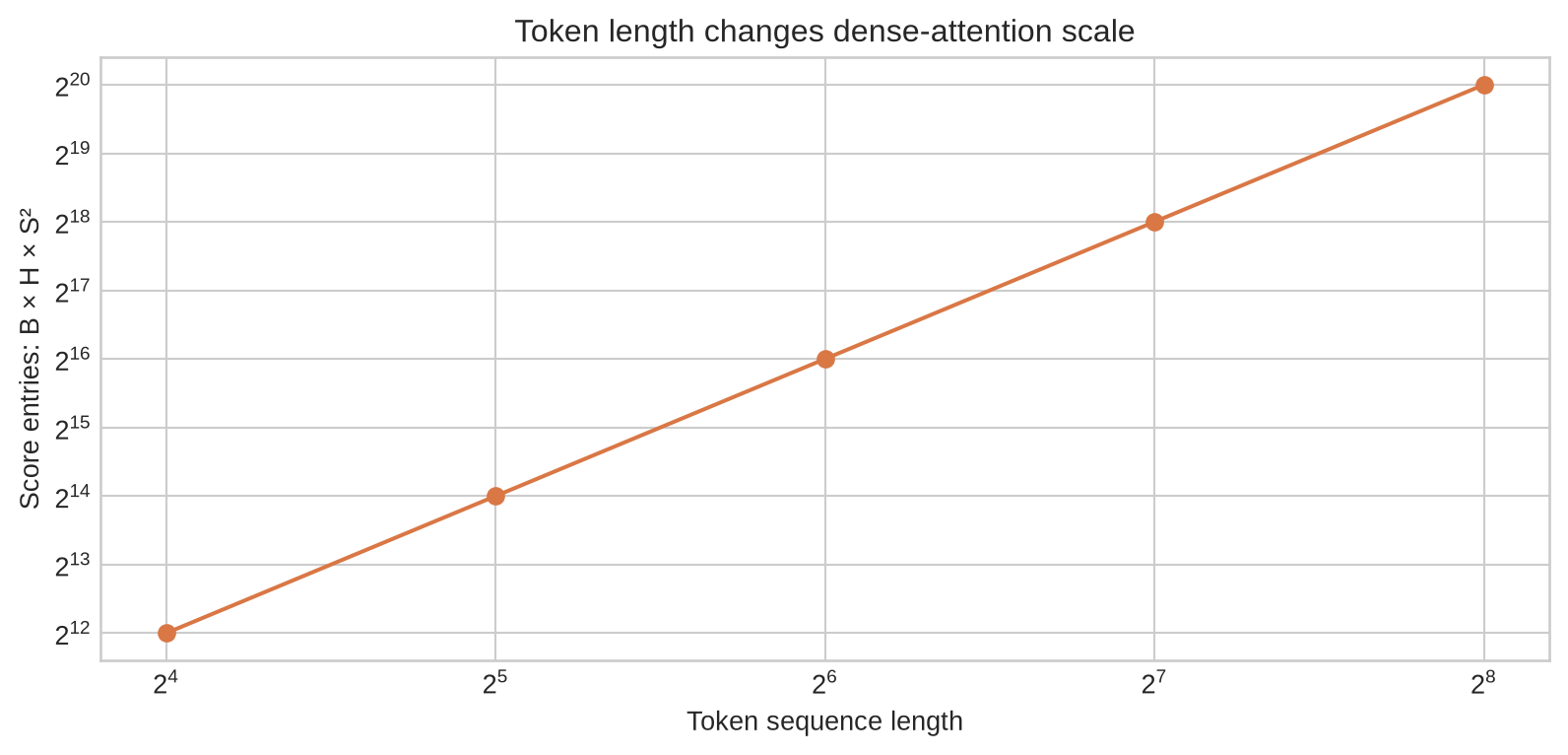
If a text becomes $S$ tokens, one batch of embeddings has shape $B\times S\times D$. Dense self-attention creates score relations proportional to $BHS^2$, for batch size $B$ and heads $H$. Splitting one linguistic unit into several tokens therefore changes both the number of embedding lookups and the number of possible attention pairs.
```{python}
#| label: fig-token-length-cost
#| fig-cap: "For dense self-attention, a tokenisation that doubles sequence length creates roughly four times as many score-matrix entries at fixed batch size and head count."
#| fig-alt: "A line chart shows attention score entries increasing quadratically for token lengths from 16 to 256."
lengths=np.array([16,32,64,128,256]); heads=8; batch=2
entries=batch*heads*lengths**2
fig,ax=plt.subplots(figsize=(8.4,4.1)); ax.plot(lengths,entries,marker="o",color=orange)
ax.set_xscale("log",base=2); ax.set_yscale("log",base=2); ax.set_xlabel("Token sequence length"); ax.set_ylabel("Score entries: B × H × S²"); ax.set_title("Token length changes dense-attention scale"); plt.tight_layout(); plt.show()
```
This accounting does not mean that the tokenizer alone determines inference cost. Width, layers, cache policy, batching, kernel choice, and decoding strategy also matter. It identifies why token-count comparisons are meaningful systems measurements and why character counts are not a reliable substitute across tokenizers.
Level 3 connected IDs to embedding rows and token counts to attention cost. Level 4 examines how vocabularies distribute that cost unevenly across languages and domains, and why the interface must be versioned with the checkpoint.
## Level 4 - Research & Systems
### Tokenisation choices distribute coverage unevenly
A vocabulary trained on one corpus or language mix may encode common forms concisely while splitting other forms into long sequences. Names, dialects, spelling variants, scripts, code, URLs, and rare morphological forms can receive disproportionate fragmentation. The resulting length increase affects context allocation, throughput, truncation risk, and the number of learning events associated with a visible string.
No general statement that one tokenizer is fair, multilingual, or robust follows from its unit type alone. Evaluation should report token counts and unknown or fallback rates by relevant language, script, domain, and input class. It should inspect the text transformations applied before segmentation and test whether important distinctions are preserved at the model boundary.
### Training and inference must use the identical interface
A model checkpoint expects the vocabulary ordering, merge rules or unigram model, normalisation policy, added-token map, maximum length, padding side, truncation side, and special-token IDs used during training. Replacing a tokenizer with another that has the same vocabulary size is incompatible: ID 14 may select a different embedding row, and the same text may have different positions and masks.
The tokenizer should therefore be versioned and loaded with the model. An audit should preserve the tokenizer artefact or exact training configuration; vocabulary hash; special-token map; normalisation and pre-tokenisation rules; byte fallback policy; maximum length; truncation and padding policy; source and target tokenizers where relevant; and token-length distributions on train, evaluation, and deployment data.
The audit should also run round-trip and boundary tests. A reversible input should satisfy an explicitly defined encode-decode comparison. Special tokens should not be inserted or removed unexpectedly. Padding should have no effect on valid-token output. Inputs at the maximum length and one position beyond it should expose the truncation or rejection policy. These tests are small, but they prevent tokenisation mismatches from appearing later as unexplained model failures.
### Text interfaces create security and evaluation boundaries
Tokenisation occurs before the model's learned computation, so a pipeline should test malformed Unicode, unusual whitespace, control characters, repeated delimiters, very long inputs, and text that is visually similar but encoded differently. These tests do not establish model safety or factual reliability. They establish that the input interface behaves as specified and that monitoring counts the same units the model actually consumes.
Token-level metrics also need interpretation. A system may have a fixed maximum number of tokens, but the amount of human-readable text that fits varies by language and segmentation. Reporting only character limits can conceal this difference; reporting only token limits can conceal the user-visible burden. Both may be required for a deployment claim.
## Common misconceptions
- **A token is always a word.** Tokens can be words, characters, bytes, subwords, or special markers.
- **Token IDs have ordinal meaning.** They are vocabulary addresses used for lookup.
- **A larger vocabulary always improves a model.** It changes coverage, table size, sequence length, data sparsity, and output cost.
- **Subword pieces are guaranteed linguistic morphemes.** Their boundaries follow the tokenisation objective and corpus statistics.
- **Padding is harmless without a mask.** Artificial positions can affect attention, loss, and pooled outputs unless excluded.
- **An unknown token and truncation do the same thing.** One replaces a unit; the other removes positions.
- **A model can use any tokenizer with the same vocabulary size.** It needs the exact ID mapping and preprocessing contract used in training.
- **A context limit in tokens means the same text length for every language.** Token counts vary with segmentation and script.
## Exercises
1. Distinguish a token string, token ID, and embedding vector in a supplied example.
2. Explain why permuting a vocabulary and embedding rows together can preserve model behaviour.
3. Segment `replaying replay` into words, characters, and the running subword inventory.
4. Calculate the embedding-table parameter count for vocabulary 50,000 and width 768.
5. Calculate the relative increase in dense score entries when token length rises from 128 to 256.
6. Implement an encoder that adds beginning and end special tokens.
7. Implement a decoder that omits padding and special tokens from displayed text.
8. Write a test that padded positions receive zero attention mass in a small causal model.
9. Give an example of a text transformation that can change a token sequence.
10. Explain why an unknown-token policy can collapse distinct strings.
11. Compare the systems consequences of word and character tokenisation for a long document.
12. Explain why BPE merge rules must be saved with a model checkpoint.
13. Design a tokenisation evaluation across two scripts or language varieties.
14. State the source and target tokenizer metadata an encoder-decoder model requires.
15. Test a tokenizer on unusual whitespace and a long repeated input.
16. State which chapter introduces the next-token probability objective.
## Summary
Tokenisation converts text into a sequence of vocabulary identifiers, and embedding lookup converts those identifiers into vectors. The vocabulary, segmentation method, special tokens, normalisation, padding, truncation, and maximum length together form a model input contract.
Word, character, byte, and subword units make different coverage, vocabulary-size, and sequence-length trade-offs. These trade-offs affect representation, attention cost, evaluation, and deployment. A tokenizer must be versioned and evaluated with the model rather than substituted at inference.
## Looking ahead
[Chapter 25](25-next-token-prediction.qmd) uses token IDs to define next-token probability distributions, training loss, and autoregressive generation.
## Further reading
Subword units based on BPE are developed by @sennrich2016bpe. SentencePiece's language-independent raw-text interface and its support for BPE and unigram segmentation are described by @kudo2018sentencepiece.