---
title: "Self-attention and Multi-head Attention"
subtitle: "Letting each position retrieve from other positions"
---
## The problem
Chapter 19 built attention as query-dependent retrieval: a decoder query scores source keys, and weighted values return a context. In that setting the query came from one sequence while the keys and values came from another. But the sequence that needs a context is often also the sequence that holds it. A word whose interpretation depends on an earlier qualifier must retrieve from that qualifier, and every position in a sequence can have such dependencies.
Self-attention answers this by using the same operation within one sequence: every position produces a query, a key, and a value, then retrieves a context from the eligible positions of that same sequence. Information from position one no longer has to pass through every intervening recurrent state to reach position five; a direct query-key comparison connects the two. One head learns one projected retrieval pattern, and multi-head attention runs several such patterns in parallel and recombines their outputs. This chapter explains those operations and deliberately stops short of a complete Transformer: positional information belongs to Chapter 21, and the residual, normalisation, and feed-forward machinery belongs to Chapter 22.
### A small constructed sequence makes retrieval visible
The running tensor has one batch item, five positions, and four input features. It is constructed to make position-to-position weights visible; the values are illustrative rather than learned language representations, and the results demonstrate retrieval mechanics.
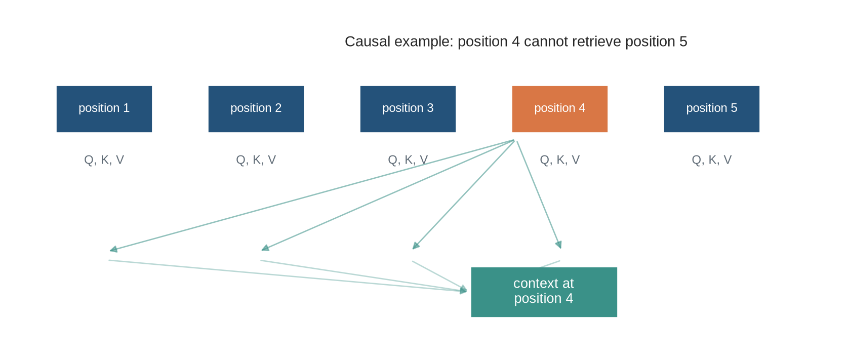
The first diagram shows one position retrieving from the rest of the sequence. Each position supplies a query, key, and value; the highlighted query at position four is scored against the eligible positions, and weighted values flow into its context. Notice that position five is absent from that mixture: the example applies a causal mask, so a position may retrieve only from itself and earlier positions.
```{python}
#| label: fig-self-attention-overview
#| fig-cap: "In self-attention, each position supplies a query, key, and value and retrieves a weighted mixture from eligible positions in the same sequence."
#| fig-alt: "Five sequence positions each emit query, key, and value arrows. One highlighted query attends to four earlier eligible positions and receives a context vector."
import numpy as np
import matplotlib.pyplot as plt
from matplotlib.patches import Rectangle, FancyArrowPatch

plt.style.use("seaborn-v0_8-whitegrid")
blue, teal, orange, purple, grey = "#24527a", "#3a9188", "#d97745", "#7a5195", "#5f6b76"
fig,ax=plt.subplots(figsize=(11,4.5)); ax.axis("off")
for i in range(5):
    x=.5+i*1.65; colour=orange if i==3 else blue
    ax.add_patch(Rectangle((x,2.6),1.05,.58,facecolor=colour,edgecolor="white")); ax.text(x+.525,2.89,f"position {i+1}",ha="center",va="center",color="white",fontsize=9)
    ax.text(x+.525,2.22,"Q, K, V",ha="center",color=grey,fontsize=9)
for i in range(4): ax.add_patch(FancyArrowPatch((5.5,2.52),(1.05+i*1.65,1.15),arrowstyle="-|>",mutation_scale=11,color=teal,alpha=.55))
ax.add_patch(Rectangle((5.0,.35),1.6,.62,facecolor=teal,edgecolor="white")); ax.text(5.8,.66,"context at\nposition 4",ha="center",va="center",color="white")
for i in range(4): ax.add_patch(FancyArrowPatch((1.05+i*1.65,1.05),(5.0,.66),arrowstyle="-|>",mutation_scale=10,color=teal,alpha=.35))
ax.text(5.5,3.65,"Causal example: position 4 cannot retrieve position 5",ha="center",fontsize=11)
ax.set_xlim(0,9); ax.set_ylim(0,4.1); plt.show()
```
The context at position four is a mixture of eligible values, not a copy of any single one. A different position forms a different query and therefore retrieves a different mixture from the same sequence, exactly as different decoder queries did in Chapter 19.
::: {.concept-box .concept-core #concept-self-attention data-term="Self-attention and multi-head attention" data-domain="Representations and Transformers"}
**Self-attention and multi-head attention.** Self-attention lets each position retrieve from eligible positions in the same sequence. Multi-head attention performs several learned retrievals in parallel. A mask defines which positions are eligible.
:::
::: {.concept-box .concept-distinction #concept-self-cross-attention data-term="Self-attention and cross-attention" data-domain="Representations and Transformers"}
**Self-attention and cross-attention.** Self-attention draws queries, keys, and values from one sequence. Cross-attention draws queries from one representation and keys and values from another, creating an explicit information boundary.
:::
## Level 1 - Intuition
### Every position asks its own retrieval question
Let $x_1,\ldots,x_S$ be the representations supplied to a self-attention layer. Position $t$ creates a query from $x_t$ and compares it with keys created from every eligible position. The resulting context at $t$ can combine information from distant positions in one layer.
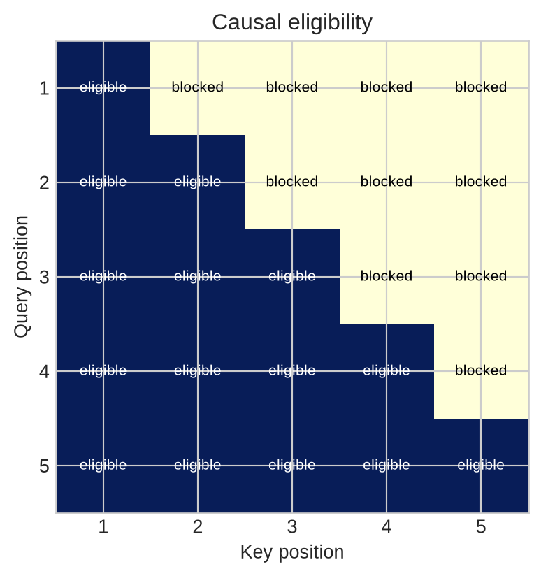
This differs from recurrence, where information at position one reaches position five only after four state transitions. It does not remove dependency constraints: a causal mask prevents position four from using position five, and positional information is still needed to distinguish sequences with the same items in different orders.
```{python}
#| label: fig-causal-mask
#| fig-cap: "A causal mask permits each position to retrieve only itself and earlier positions."
#| fig-alt: "A lower-triangular five-by-five eligibility matrix has rows as query positions and columns as key positions; future positions are greyed out."
length=5
mask=np.tril(np.ones((length,length),dtype=bool))
fig,ax=plt.subplots(figsize=(5.2,4.4)); ax.imshow(mask,cmap="YlGnBu",vmin=0,vmax=1)
for i in range(length):
    for j in range(length): ax.text(j,i,"eligible" if mask[i,j] else "blocked",ha="center",va="center",fontsize=8,color="white" if mask[i,j] else "black")
ax.set_xticks(range(length),range(1,length+1)); ax.set_yticks(range(length),range(1,length+1)); ax.set_xlabel("Key position"); ax.set_ylabel("Query position"); ax.set_title("Causal eligibility")
plt.tight_layout(); plt.show()
```
### Projections separate matching from retrieved content
The input representation is not used directly for all three roles. Learned matrices project it into query, key, and value spaces. Queries and keys determine which positions match; values determine what content is returned. Separate projections allow a model to use one feature direction for matching and another for retrieved information.
The names describe a retrieval analogy, not three kinds of token. A query asks what the present position needs; a key says what a position can be matched on; a value is the information offered if that position is selected. Consider a word whose interpretation depends on an earlier qualifier. Its query can favour keys that mark a relevant qualifier, while the retrieved value carries the representation that changes the present context. Which feature plays each role is learned from the training objective. The same input position therefore supplies all three, but through different learned projections.
The distinction also prevents a common error. A high score does not mean that a key vector is copied into the output. Scores determine weights; the output is a weighted mixture of value vectors. A model can match positions on one property and retrieve a different property from them.
### Heads provide several retrieval subspaces
One head produces one set of weights and one context vector per position. Multi-head attention uses several independently parameterised projections. A head can learn a local, long-range, syntactic, or domain-specific pattern if that helps the objective, but no such role is guaranteed by the head number.
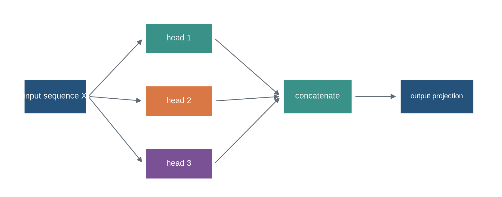
At fixed model width, multi-head attention is not simply "more attention". It divides the internal feature width into several smaller projected spaces, runs a retrieval calculation in each one, and lets a later output projection mix the results. The useful claim is modest: several learned comparison spaces can represent different routing patterns at the same layer. Whether they do so is an empirical question.
```{python}
#| label: fig-multi-head-overview
#| fig-cap: "Multi-head attention applies several projected self-attention operations in parallel, concatenates their contexts, and projects the result back to model width."
#| fig-alt: "An input sequence branches into three labelled heads, each produces a context sequence, then the outputs concatenate and pass through one output projection."
fig,ax=plt.subplots(figsize=(11,4.2)); ax.axis("off")
ax.add_patch(Rectangle((.4,1.55),1.35,.68,facecolor=blue,edgecolor="white")); ax.text(1.075,1.89,"input sequence X",ha="center",va="center",color="white")
for i,y in enumerate([3.05,1.8,.55]):
    ax.add_patch(FancyArrowPatch((1.8,1.89),(3.0,y),arrowstyle="-|>",mutation_scale=13,color=grey))
    ax.add_patch(Rectangle((3.05,y-.3),1.45,.6,facecolor=[teal,orange,purple][i],edgecolor="white")); ax.text(3.775,y,f"head {i+1}",ha="center",va="center",color="white")
    ax.add_patch(FancyArrowPatch((4.55,y),(6.0,1.89),arrowstyle="-|>",mutation_scale=13,color=grey))
ax.add_patch(Rectangle((6.05,1.55),1.5,.68,facecolor=teal,edgecolor="white")); ax.text(6.8,1.89,"concatenate",ha="center",va="center",color="white")
ax.add_patch(FancyArrowPatch((7.6,1.89),(8.55,1.89),arrowstyle="-|>",mutation_scale=13,color=grey))
ax.add_patch(Rectangle((8.6,1.55),1.6,.68,facecolor=blue,edgecolor="white")); ax.text(9.4,1.89,"output projection",ha="center",va="center",color="white",fontsize=9)
ax.set_xlim(0,10.7); ax.set_ylim(0,3.7); plt.show()
```
```{python}
#| label: fig-head-patterns
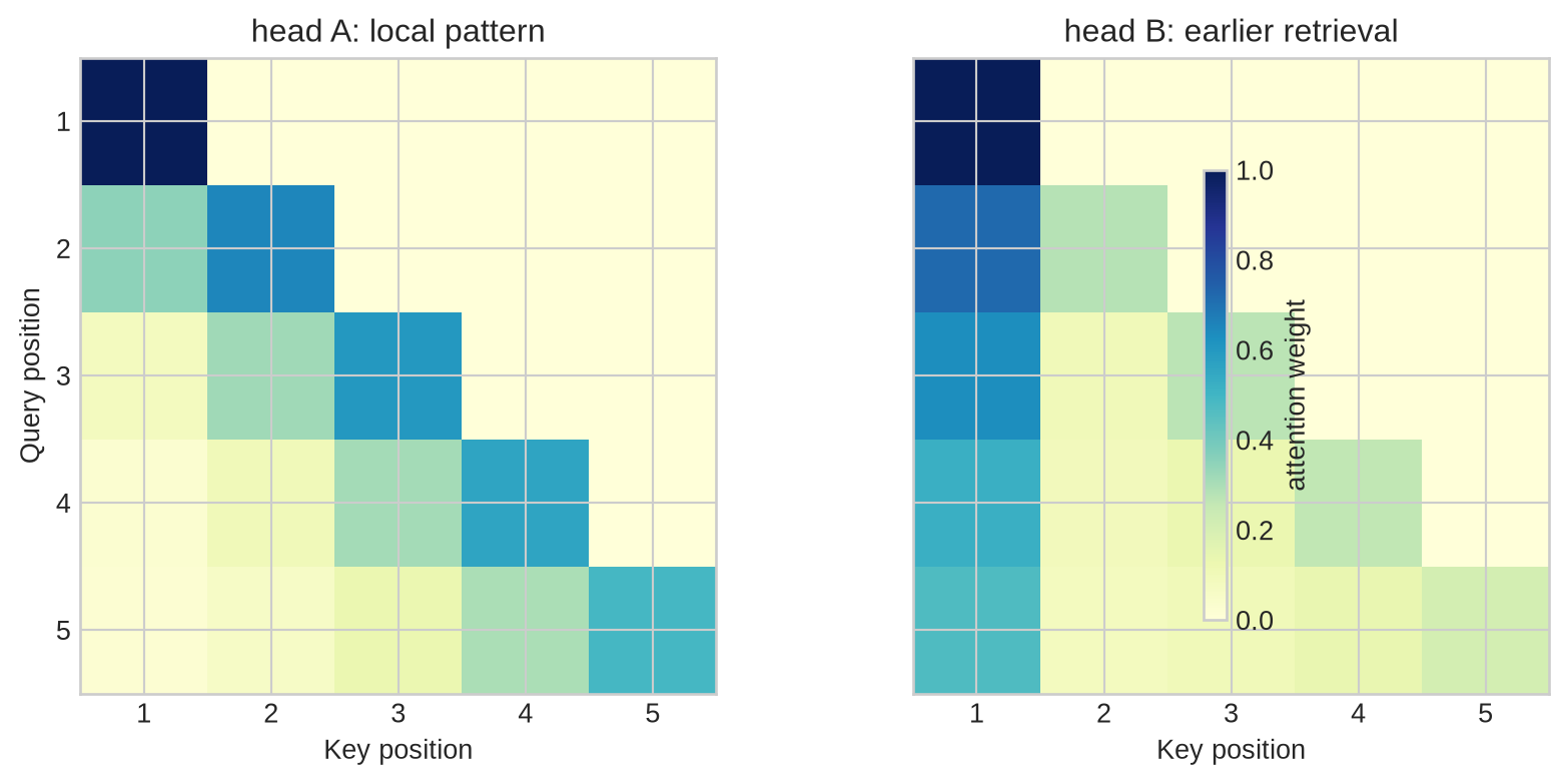
#| fig-cap: "Two heads can assign different eligible attention patterns to the same positions; these patterns are learned behaviours, not labels with guaranteed meanings."
#| fig-alt: "Two side-by-side lower-triangular heatmaps. The first emphasises nearby positions; the second emphasises the first position and selected earlier positions."
local=np.array([[1,0,0,0,0],[.35,.65,0,0,0],[.08,.32,.60,0,0],[.03,.10,.31,.56,0],[.02,.06,.13,.30,.49]])
retrieve=np.array([[1,0,0,0,0],[.72,.28,0,0,0],[.63,.10,.27,0,0],[.52,.09,.13,.26,0],[.47,.08,.10,.14,.21]])
fig,axes=plt.subplots(1,2,figsize=(9,3.8),sharey=True)
for ax,a,title in zip(axes,[local,retrieve],["head A: local pattern","head B: earlier retrieval"]):
    im=ax.imshow(a,cmap="YlGnBu",vmin=0,vmax=1); ax.set_title(title); ax.set_xlabel("Key position"); ax.set_xticks(range(5),range(1,6)); ax.set_yticks(range(5),range(1,6))
axes[0].set_ylabel("Query position"); fig.colorbar(im,ax=axes,shrink=.8,label="attention weight"); plt.tight_layout(); plt.show()
```
The figure is deliberately synthetic. It shows a possibility, not evidence that a trained head has a stable semantic identity. In particular, the output projection can combine or cancel information from multiple heads, so an attention map is a diagnostic object rather than a complete explanation of a prediction.
Level 1 defined the operation. Level 2 follows the matrix products and mask through one attention head.
## Level 2 - Mechanics
### Scaled dot products create one score row per query
For input $X\in\mathbb{R}^{S\times D}$, one head projects
$$Q=XW_Q,\quad K=XW_K,\quad V=XW_V.$$
The score matrix is $QK^\top$. Entry $(t,j)$ compares query position $t$ with key position $j$. Scaled dot-product attention uses
$$A=\operatorname{softmax}\left(\frac{QK^\top}{\sqrt{D_k}}+M\right),\qquad C=AV,$$
where softmax is applied across keys and $M$ encodes eligibility. The division by $\sqrt{D_k}$ controls score scale as key width changes [@vaswani2017].
```{python}
X=np.array([[1.,0.,.2,.1],[.8,.2,.1,.3],[.1,.9,.3,.2],[.3,.4,.8,.2],[.2,.1,.6,.9]])
Wq=np.array([[.7,0.],[.1,.6],[.2,.4],[.4,.1]])
Wk=np.array([[.5,.2],[.2,.7],[.6,.1],[.1,.5]])
Wv=np.array([[.4,.1,.2],[.2,.5,.1],[.1,.3,.6],[.5,.2,.2]])
Q,K,V=X@Wq,X@Wk,X@Wv
scores=Q@K.T/np.sqrt(Q.shape[-1])
def row_softmax(z):
    z=z-z.max(axis=-1,keepdims=True); ez=np.exp(z); return ez/ez.sum(axis=-1,keepdims=True)
weights=row_softmax(scores); contexts=weights@V
print("Q, K, V:",Q.shape,K.shape,V.shape)
print("scores, weights, contexts:",scores.shape,weights.shape,contexts.shape)
print("row sums:",weights.sum(axis=-1).round(6))
```
Each row of `weights` is a separate distribution. Softmax over columns makes a query's eligible keys compete. Softmax over rows would create a different and usually unintended model.
The context $C_t$ is the attention contribution for position $t$, not yet a complete Transformer-layer output. A full Transformer block also retains the position's prior representation through a residual path, normalises appropriate axes, and applies a position-wise feed-forward transformation. Those components are intentionally deferred to Chapter 22, so that the retrieval operation remains visible here.
### Causal and padding masks combine by exclusion
A causal mask blocks future key positions. A padding mask blocks positions that do not contain source data. Both act on score entries before softmax. For a batch, the padding mask is broadcast over query positions; the causal mask is broadcast over batch items and heads.
```{python}
causal=np.tril(np.ones((5,5),dtype=bool))
valid_keys=np.array([True,True,True,True,False])
eligible=causal & valid_keys[None,:]
masked_scores=np.where(eligible,scores,-np.inf)
masked_weights=row_softmax(masked_scores)
print("masked weight at query 4:",masked_weights[3].round(3))
print("future mass at query 2:",masked_weights[1,2:].sum())
```
An all-masked query row requires an explicit policy. It may arise from malformed lengths or empty examples. Letting it become NaN hides an input-contract failure.
Mask orientation matters. In the displayed matrices, rows are queries and columns are keys, so a causal mask is lower triangular: query four may use keys one through four. Some libraries use different argument names or boolean conventions, where `True` can mean either *keep* or *block*. A tiny hand-checked example and a future-perturbation test are safer than copying a mask expression without checking its contract.
### Heads split width, not sequence responsibility
With model width $D$ and $H$ heads, many implementations use head width $d_h=D/H$. Each head has its own $W_Q^{(h)}, W_K^{(h)}, W_V^{(h)}$. Contexts concatenate along features and an output projection maps them back to width $D$.
Splitting width does not allocate different token positions to each head. Every head usually sees the same eligible positions. It receives different projected coordinates, so its scores and retrieved mixtures can differ.
For example, with $D=512$ and $H=8$, a conventional implementation uses $d_h=64$. Each head still produces a score for every allowed query-key pair; it has fewer coordinates in which to construct that score. The concatenated head outputs recover width 512 before the output projection. Other designs use unequal widths or grouped key/value projections, but the shape contract must be made explicit rather than inferred from the word "head".
Level 2 followed the projections, scores, and masks of one head. Level 3 expresses the batched multi-head computation in tensor form and tests the information boundary of an implementation.
## Level 3 - Mathematics & Code
### Batched multi-head shapes make the contracts explicit
For $X\in\mathbb{R}^{B\times S\times D}$, reshape projections into $B\times H\times S\times d_h$. The score tensor then has shape $B\times H\times S\times S$. Its last axis is keys; its penultimate axis is queries.
```{python}
import torch
from torch import nn

torch.manual_seed(20)
B,S,D,H=2,5,8,2; d_h=D//H
x=torch.randn(B,S,D)
qkv=nn.Linear(D,3*D,bias=False)(x)
q,k,v=qkv.chunk(3,dim=-1)
def split_heads(t): return t.view(B,S,H,d_h).transpose(1,2)
q,k,v=map(split_heads,(q,k,v))
scores=torch.matmul(q,k.transpose(-2,-1))/np.sqrt(d_h)
causal_mask=torch.tril(torch.ones(S,S,dtype=torch.bool))
scores=scores.masked_fill(~causal_mask,-torch.inf)
attention=torch.softmax(scores,dim=-1)
head_context=torch.matmul(attention,v)
merged=head_context.transpose(1,2).contiguous().view(B,S,D)
print("scores:",tuple(scores.shape),"attention:",tuple(attention.shape))
print("merged output:",tuple(merged.shape),"masked mass:",attention[0,0,1,2:].sum().item())
```
The `transpose` changes the logical axis order. `contiguous()` makes the requested feature merge explicit before `view`. The output projection, omitted here for visibility, is another learned linear layer and does not change the sequence length.
### Scaling controls score variance
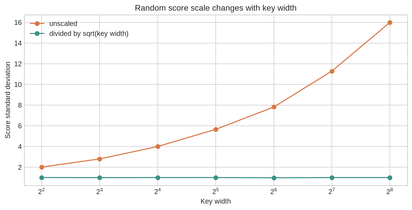
If independent query and key coordinates have zero mean and unit variance, an unscaled dot product has variance proportional to $D_k$. Larger key widths can therefore make softmax excessively concentrated early in training. Dividing by $\sqrt{D_k}$ keeps the scale closer to constant under those assumptions.
```{python}
#| label: fig-score-scaling
#| fig-cap: "Scaling dot products by the square root of key width keeps typical score variation comparable as width increases."
#| fig-alt: "Two line plots show the standard deviation of unscaled and scaled random dot products across key widths from 4 to 256."
rng=np.random.default_rng(20); widths=np.array([4,8,16,32,64,128,256]); raw=[]; scaled=[]
for width in widths:
    dots=(rng.normal(size=(4000,width))*rng.normal(size=(4000,width))).sum(axis=1)
    raw.append(dots.std()); scaled.append((dots/np.sqrt(width)).std())
fig,ax=plt.subplots(figsize=(8.5,4.4)); ax.plot(widths,raw,marker="o",color=orange,label="unscaled"); ax.plot(widths,scaled,marker="o",color=teal,label="divided by sqrt(key width)")
ax.set_xscale("log",base=2); ax.set_xlabel("Key width"); ax.set_ylabel("Score standard deviation"); ax.set_title("Random score scale changes with key width"); ax.legend(); plt.tight_layout(); plt.show()
```
This is a distributional argument about initial scores, not a guarantee about trained representations. Learned norms, normalisation, precision, and masks also affect score scale.
### A module test should assert information boundaries
```{python}
class CausalSelfAttention(nn.Module):
    def __init__(self,width,heads):
        super().__init__(); self.width=width; self.heads=heads; self.head_width=width//heads
        self.qkv=nn.Linear(width,3*width); self.out=nn.Linear(width,width)
    def forward(self,x):
        b,s,_=x.shape; q,k,v=self.qkv(x).chunk(3,dim=-1)
        def split(t): return t.view(b,s,self.heads,self.head_width).transpose(1,2)
        q,k,v=map(split,(q,k,v)); score=(q@k.transpose(-2,-1))/np.sqrt(self.head_width)
        mask=torch.tril(torch.ones(s,s,device=x.device,dtype=torch.bool)); score=score.masked_fill(~mask,-torch.inf)
        a=torch.softmax(score,dim=-1); c=(a@v).transpose(1,2).contiguous().view(b,s,self.width)
        return self.out(c),a

layer=CausalSelfAttention(8,2); base=torch.randn(1,5,8); changed=base.clone(); changed[:,4]+=100
out_base,_=layer(base); out_changed,_=layer(changed)
print("earlier outputs unchanged:",torch.allclose(out_base[:,:4],out_changed[:,:4],atol=1e-6))
```
The perturbation test checks a causal promise: changing a future input cannot alter earlier outputs. It is stronger than inspecting a triangular plot because it tests the complete implemented path.
Level 3 established self-attention as a testable batched module. Level 4 examines what the all-pairs access pattern costs, how head patterns may and may not be interpreted, and how inference avoids repeated projection work.
## Level 4 - Research & Systems
### Self-attention exchanges sequential depth for all-pairs work
All sequence positions can form queries, keys, and values in parallel. Full self-attention then compares every query-key pair. For length $S$, the score matrix has $S^2$ entries per head and batch item. This permits direct interaction between distant positions in one layer but produces quadratic memory and arithmetic in sequence length [@vaswani2017].
For a dense score tensor the element count is $BHS^2$. At four-byte floating point precision, scores alone require roughly $4BHS^2$ bytes before accounting for weights, gradients, activations, projections, and framework overhead. This accounting is why a change from length 1,024 to 8,192 is not an eight-fold enlargement of dense attention: the score relation is sixty-four times larger.
Flash-style kernels, blockwise computation, sparse patterns, and approximate methods can reduce materialised memory or restrict pair sets. Their equivalence conditions, mask semantics, numerical tolerances, and hardware dependence must be stated; an implementation that changes eligible pairs changes the model.
### Multi-head patterns require tests before interpretation
Head maps can reveal routing patterns or implementation errors, especially masked mass, repeated rows, dead heads, and unexpectedly uniform distributions. They do not assign a semantic role to a head or establish causal explanation. Heads can be redundant, later projections can mix them, and removing one head can trigger compensation elsewhere.
Interventions should vary a source value, a head output, or a selected edge while holding the relevant rest of the model fixed, then measure the output change. Even then, a local intervention does not establish a global natural-language explanation.
### Autoregressive inference caches prior keys and values
In causal generation, recomputing keys and values for every earlier position at each new token repeats work. A key-value cache retains projected keys and values from prior positions. Each new query attends to the cache plus its current key and value. The cache lowers repeated projection work but grows linearly with generated length, layers, heads, batch size, and value width.
The cache is not a separate memory of text: it is a collection of projected tensors with a specific model checkpoint, layer, dtype, position convention, and mask history. Chapter 27 examines this inference contract and its memory consequences in more detail.
### A self-attention audit records eligibility and cost
An audit should record model width, heads, head width, all projection shapes, scale factor, softmax axis, causal and padding masks, all-masked-row policy, dropout, dtype, score ranges, attention entropy, masked mass, sequence lengths, cache policy, peak memory, and valid-token throughput. It should test causal invariance, padding invariance, shape contracts, and numerical agreement with a small reference implementation.
## Common misconceptions
- **Self-attention knows order from token embeddings alone.** It needs order encoded in its input or a separate positional mechanism.
- **Each head attends to a different subset of tokens by design.** Heads usually receive the same eligible positions with different learned projections.
- **Causal masking means all positions receive the same context.** Each query row has a different eligible prefix and different scores.
- **The scale factor makes attention stable in every setting.** It addresses one score-variance mechanism under stated assumptions.
- **Multi-head attention is several independent models.** Heads are recombined by an output projection and trained jointly.
- **A triangular heatmap proves causal implementation.** A perturbation test must include all code paths.
- **Full self-attention has linear memory in sequence length.** Its dense score relations are quadratic.
- **A key-value cache removes attention cost.** It avoids repeated projections but each new query still scores cached keys.
## Exercises
1. State the shapes of $Q$, $K$, $V$, scores, weights, and output for batch 4, length 32, width 128, and eight heads.
2. Draw causal eligibility for six positions and count eligible pairs.
3. Verify that softmax operates over keys in a supplied score tensor.
4. Implement a padding mask and test zero masked mass.
5. Explain why causal and padding masks can both apply to one score entry.
6. Derive the variance of an unscaled random dot product under independent unit-variance coordinates.
7. Reproduce the scaling figure for non-unit coordinate variance.
8. Implement the omitted output projection in the batched example.
9. Compare one-head and four-head parameter counts at fixed model width.
10. Write a causal perturbation test for a batched implementation.
11. Measure score-matrix elements for lengths 128, 512, 2,048, and 8,192.
12. Estimate key-value cache bytes for a specified layer count, head width, and generated length.
13. Design a test for an all-masked input row.
14. Compare a dense reference implementation with a framework attention kernel on a small tensor.
15. Design an intervention that tests a claim about one attention head.
16. Explain which additional mechanism is needed before self-attention can distinguish reversed sequences.
## Summary
Self-attention uses every sequence position as a query, key, and value source. Scaled dot products create one score distribution over eligible keys for every query position, and weighted value sums produce new contextual representations. Causal and padding masks define the information boundary.
Multi-head attention repeats this retrieval operation in several learned projection spaces, concatenates the resulting contexts, and projects them back to model width. It permits direct long-range interaction but creates a dense query-key relation whose cost grows quadratically with length.
## Looking ahead
[Chapter 21](21-positional-information.qmd) supplies positional information, allowing non-recurrent self-attention to distinguish sequence order explicitly. [Chapter 22](22-transformer-block.qmd) then places attention inside a complete Transformer block.
## Further reading
Scaled dot-product and multi-head attention are introduced by @vaswani2017. The general attention operation and its alignment-based origins are covered in @bahdanau2015attention and @luong2015attention.