---
title: "Inference-time Scaling"
subtitle: "Sampling, voting, verification, and the conditions under which more computation helps"
---
## Chapter orientation
### Why this chapter matters
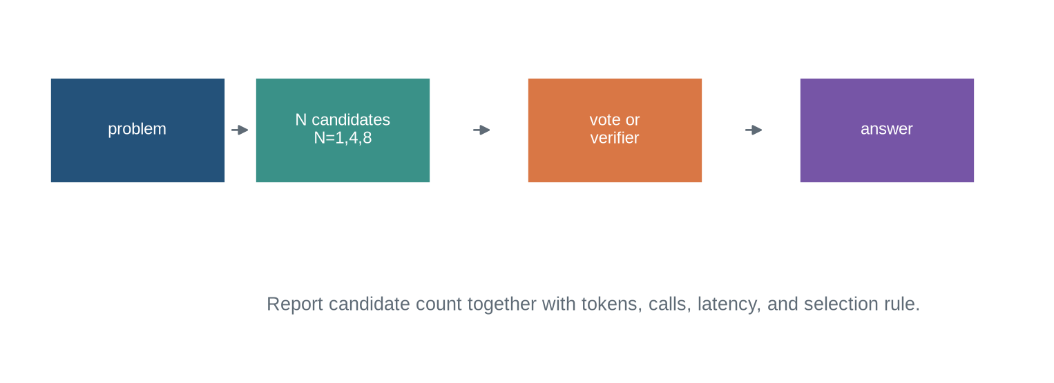
Inference-time scaling allocates more computation to a problem after a model has been trained. A system can sample several solutions, vote over answers, use a verifier to select a candidate, search a tree of partial solutions, or spend additional tokens refining a response. Performance can improve when the extra computation produces useful candidate diversity and a selection signal can identify better candidates. It can also plateau, amplify a shared error, or cost more than the task warrants.
This chapter develops controlled comparisons between compute budgets. It does not assume that best-of-N sampling, self-consistency, or verification helps every problem. Chapter 38 studies refinement and search loops; Chapter 39 turns to training policies with reasoning rewards.
### Learning objectives
By the end of this chapter, you should be able to:
- define inference-time scaling and a compute budget;
- implement best-of-N and majority-vote selection on toy candidates;
- calculate the probability that at least one of several independent samples is correct;
- explain why sample independence and selection quality limit scaling gains;
- plot accuracy against tokens, calls, latency, or monetary cost; and
- design a controlled scaling experiment with fixed model, task, and selection rule.
### Running candidates
For a checkable problem, a system samples several candidate answers. A vote or verifier selects one. Increasing the number of samples increases cost and can increase the chance that at least one candidate is correct.
```{python}
#| label: fig-scaling-loop
#| fig-cap: "Inference-time scaling increases a candidate or search budget, then uses a declared vote or verifier to select an answer."
#| fig-alt: "A prompt produces one, four, or eight candidates, which pass to a selector and then an answer with a recorded cost."
import numpy as np
import matplotlib.pyplot as plt
from matplotlib.patches import Rectangle, FancyArrowPatch
plt.style.use("seaborn-v0_8-whitegrid")
blue,teal,orange,purple,grey="#24527a","#3a9188","#d97745","#7655a6","#5f6b76"
fig,ax=plt.subplots(figsize=(10,3.5)); ax.axis("off")
for x,label,c in [(.3,"problem",blue),(2.0,"N candidates\nN=1,4,8",teal),(4.25,"vote or\nverifier",orange),(6.5,"answer",purple)]: ax.add_patch(Rectangle((x,1.3),1.45,.62,facecolor=c,edgecolor="white")); ax.text(x+.725,1.61,label,ha="center",va="center",color="white",fontsize=9)
for x in [1.78,3.78,6.03]: ax.add_patch(FancyArrowPatch((x,1.61),(x+.2,1.61),arrowstyle="-|>",color=grey,mutation_scale=11))
ax.text(4.8,.55,"Report candidate count together with tokens, calls, latency, and selection rule.",ha="center",color=grey); ax.set_xlim(0,8.5); ax.set_ylim(.2,2.3); plt.show()
```
::: {.concept-box .concept-core #concept-inference-time-scaling data-term="Inference-time scaling" data-domain="Reasoning models"}
**Inference-time scaling.** Changing task performance by allocating more computation after training, for example through sampling, voting, verification, or search. Its evidence must include candidate count, selection rule, cost, and task-specific outcome.
:::
## Level 1 - Intuition
### More attempts can raise coverage
If a single sampled solution has probability \(p\) of being correct and samples are independent, the probability that at least one among \(N\) is correct is \(1-(1-p)^N\). This is an upper-bound intuition for best-of-N: the system still needs to recognise or select the correct candidate. Correlated mistakes, narrow decoding, and weak selectors reduce the practical gain.
```{python}
p=.35
for n in [1,2,4,8]: print(n,"independent coverage",round(1-(1-p)**n,3))
```
Sampling does not create new evidence. It produces several continuations of the same model under the same context. If all candidates repeat a common misconception, a majority vote can reinforce it. If a verifier checks the relevant property, it can select a rare correct candidate. The mechanism must be evaluated on the task rather than inferred from candidate count.
```{python}
candidates=[12,13,12,11,12]
print("majority answer:",max(set(candidates),key=candidates.count))
```
### Independence is an assumption, not a decoding setting
The coverage expression assumes that each draw succeeds independently with the same probability. Model samples rarely meet that condition. The same prompt, context, model weights, and high-probability tokens can produce near-duplicate continuations. Lowering temperature can make repetition more likely; raising it can produce candidates that are different but less likely to satisfy the task. Changing the prompt between samples may increase diversity, but then the scaling comparison includes a prompt ensemble rather than a fixed prompting policy.
Measure dependence from the candidates produced, not from the requested sample count. Useful diagnostics include duplicate-answer rate, answer entropy after normalisation, pairwise agreement, and the proportion of items for which every candidate gives the same wrong answer. These records identify whether a larger budget added coverage or simply repeated the same trajectory. They also establish the conditions under which the independent-coverage calculation is a teaching approximation rather than an empirical prediction.
## Level 2 - Selection methods
### Best-of-N needs a score with useful ranking power
Best-of-N generates \(N\) candidates and chooses the highest-scoring one. The score can be an exact verifier, a learned reward, a self-evaluation, or a task-specific heuristic. An oracle score that knows the answer provides a useful educational upper bound but is not a deployable selection rule. A learned scorer requires its own precision, recall, and distribution-shift evaluation from Chapter 36.
```{python}
candidates=[{"answer":12,"score":.91},{"answer":13,"score":.63},{"answer":11,"score":.42}]
selected=max(candidates,key=lambda row:row["score"])
print("selected:",selected)
```
### The oracle gap bounds a selection claim
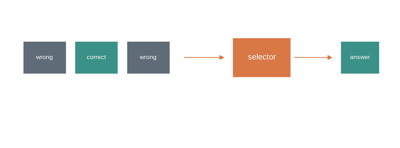
For each candidate set, an oracle selector chooses a correct candidate whenever one exists. It therefore measures coverage, not deployable performance. The difference between oracle-selected accuracy and the system's actual selected accuracy is the selection gap. A large gap indicates that more candidate generation may still be useful if the system can obtain a better verifier or ranking signal. A small gap with low oracle accuracy indicates that the main limitation is candidate generation under the current budget.
This decomposition prevents two opposite errors. An oracle result should not be reported as an achievable system result, because the oracle has access to the answer that deployment lacks. Conversely, a weak learned selector should not be used to conclude that sampling itself has no value when correct candidates were present but discarded. Verifier-guided reasoning makes this distinction practical: the value of a verifier depends on how it ranks the candidate set it actually receives [@cobbe2021training].
```{python}
#| label: fig-coverage-selection
#| fig-cap: "Candidate coverage and selection accuracy are separate: a correct candidate helps only when the selection rule retains it."
#| fig-alt: "A two-stage diagram shows several candidates including one correct candidate, then a selector that may choose correct or incorrect output."
fig,ax=plt.subplots(figsize=(9,3.2)); ax.axis("off")
for i,(label,c) in enumerate([("wrong",grey),("correct",teal),("wrong",grey)]): ax.add_patch(Rectangle((.4+i*1.2,1.4),1,.48,facecolor=c,edgecolor="white")); ax.text(.9+i*1.2,1.64,label,ha="center",va="center",color="white",fontsize=8)
ax.add_patch(FancyArrowPatch((4.1,1.64),(5.1,1.64),arrowstyle="-|>",color=orange,mutation_scale=12)); ax.add_patch(Rectangle((5.25,1.35),1.35,.58,facecolor=orange,edgecolor="white")); ax.text(5.93,1.64,"selector",ha="center",va="center",color="white")
ax.add_patch(FancyArrowPatch((6.65,1.64),(7.6,1.64),arrowstyle="-|>",color=orange,mutation_scale=12)); ax.add_patch(Rectangle((7.75,1.4),.9,.48,facecolor=teal,edgecolor="white")); ax.text(8.2,1.64,"answer",ha="center",va="center",color="white",fontsize=8)
ax.set_xlim(0,9); ax.set_ylim(.4,2.4); plt.show()
```
### Self-consistency votes over answers
Self-consistency samples several reasoning paths and selects the most common final answer. It can help when correct paths converge on a shared answer while errors are diverse [@wang2022self]. It fails when candidates share a systematic error, when answer extraction is ambiguous, or when an answer requires evidence rather than a stable vote. The grouping rule for equivalent answers must be explicit.
```{python}
answers=["12","12","twelve","13","12"]
normalised=[a.lower().replace("twelve","12") for a in answers]
print("vote:",max(set(normalised),key=normalised.count))
```
### Votes need an equivalence rule and a policy for disagreement
Voting operates on grouped answers, not raw strings. The grouping may parse integers, canonicalise algebraic expressions, compare executable outputs, or apply a task-specific normaliser. A loose normaliser can merge distinct answers; a strict one can split equivalent answers and discard the vote's intended signal. Store the raw candidate, normalised answer, and any parse failure so that the grouping can be inspected.
A vote can tie, distribute its mass across many answers, or return an answer supported by only a small share of candidates. The system needs a predeclared response: choose a tie-breaker, generate more candidates up to a budget, invoke a verifier, abstain, or return the answer with an uncertainty flag. The result should report the frequency of these conditions. Selecting the first answer that wins after an undeclared manual inspection converts a scaling experiment into an untracked selection procedure.
## Level 3 - Curves and controls
### A scaling curve needs matched conditions
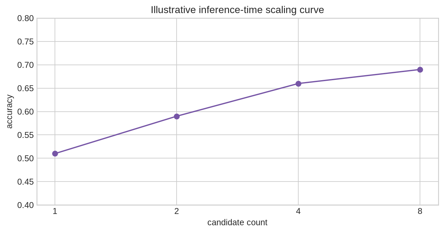
Hold the checkpoint, tokenizer, prompt template, task set, maximum candidate length, decoding distribution, and evaluator fixed while changing the compute budget. Then report mean outcome, uncertainty, total generated tokens, model calls, verifier calls, latency, and cost. If a larger budget also uses a different prompt or a stronger verifier, the result does not isolate inference-time scaling.
Sampling adds randomness, so one run at each budget is a weak basis for a curve. Use repeated draws or record seeds and report variation across them when feasible. The purpose is not to manufacture a precise estimate from a small benchmark; it is to show whether the apparent ordering of budgets persists under the stated sampling policy.
```{python}
budgets=np.array([1,2,4,8]); accuracy=np.array([.51,.59,.66,.69]); tokens=budgets*220
for n,a,t in zip(budgets,accuracy,tokens): print({"samples":int(n),"accuracy":a,"tokens":int(t)})
```
```{python}
#| label: fig-accuracy-compute
#| fig-cap: "An inference-time scaling result reports outcome accuracy against a declared compute budget and shows diminishing gains where they occur."
#| fig-alt: "A curve plots illustrative accuracy against candidate count one, two, four, and eight, with a second axis for token cost."
fig,ax=plt.subplots(figsize=(7.5,4)); ax.plot(budgets,accuracy,marker="o",color=purple); ax.set_xscale("log",base=2); ax.set_xticks(budgets,[str(x) for x in budgets]); ax.set_xlabel("candidate count"); ax.set_ylabel("accuracy"); ax.set_ylim(.4,.8); ax.set_title("Illustrative inference-time scaling curve"); plt.tight_layout(); plt.show()
```
### Candidate count is not a complete compute budget
Two systems that each sample eight candidates can use very different resources. Candidate length, context length, decoding parameters, model size, precision, tool calls, verifier cost, batching, and parallel execution all change latency and cost. Generated tokens are a useful common unit for some comparisons, but they omit input processing, cache reuse, external computation, and hardware utilisation. Wall-clock latency is the relevant constraint for an interactive service, while total accelerator time can matter more for capacity planning.
Choose the primary budget measure before inspecting the curve, then retain the other measures as supporting records. For example, an interactive mathematical assistant may set a p95 latency ceiling and report tokens and verifier calls under that ceiling. An offline data-cleaning system may instead set a total compute or monetary budget. The choice is a deployment decision, not a property of the model; Chapter 48 will treat the broader serving consequences.
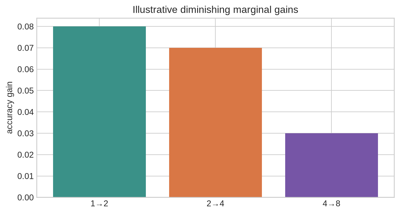
The curve can flatten because candidate quality is low, errors are correlated, the verifier is weak, or the task already saturates at one pass. A negative result is informative: it identifies a budget that adds cost without improving the measured outcome.
Scaling curves should also be reported by task slice. Arithmetic with an exact verifier, multi-step questions with ambiguous answer extraction, and long-context tasks with substantial input cost can have different frontiers even when their pooled accuracy is similar. A budget chosen from an aggregate curve may spend most of its additional computation on items that already saturate while leaving the relevant failures unchanged. The item-level record from Chapter 36 allows the curve to be decomposed without changing the evaluation after results are known.
```{python}
#| label: fig-marginal-gain
#| fig-cap: "Marginal accuracy gain per additional candidate can fall as an inference-time budget rises, making a smaller budget preferable for some deployments."
#| fig-alt: "Bars show decreasing illustrative marginal accuracy gains from one to two, two to four, and four to eight candidates."
gains=np.diff(accuracy); labels=["1→2","2→4","4→8"]
fig,ax=plt.subplots(figsize=(6.8,3.7)); ax.bar(labels,gains,color=[teal,orange,purple]); ax.set_ylabel("accuracy gain"); ax.set_title("Illustrative diminishing marginal gains"); plt.tight_layout(); plt.show()
```
### A scaling policy needs a stopping rule
Sampling can stop at a fixed candidate count, after an exact verifier accepts a result, when a vote margin reaches a threshold, or when a cost or latency limit is reached. Each rule changes the distribution of computation across inputs. Stopping after the first accepted candidate may be efficient when the verifier is reliable, but it can introduce order effects when early candidates are systematically easier to accept. A fixed budget is easier to compare; an adaptive stopping rule can be more efficient if it is evaluated as a policy rather than reported as a single average.
Record the stopping event for each item. The rate of verification acceptance, timeout, tie, exhausted budget, and abstention shows how the policy behaved. If an evaluation silently retries only the items that fail at a small budget, its reported large-budget accuracy no longer describes the policy that would run in deployment.
## Level 4 - Audit and limits
### Budgets should be adaptive only under a declared rule
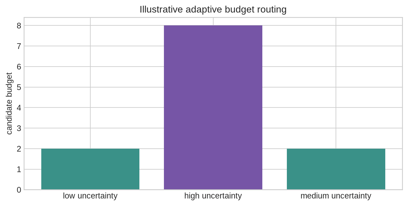
An adaptive system can allocate more samples to uncertain or difficult inputs. It then needs a routing rule and an evaluation that reports performance by route. Sending only failed cases to a large budget after viewing their answers would overstate an online system's performance. The trigger must use information available before the final answer is known.
```{python}
uncertainty=np.array([.12,.66,.31])
budgets=np.where(uncertainty>.5,8,2)
print("allocated sample budgets:",budgets)
```
```{python}
#| label: fig-adaptive-routing
#| fig-cap: "An adaptive inference policy routes inputs to smaller or larger budgets using an observable pre-answer signal such as uncertainty."
#| fig-alt: "Three inputs with low, high, and medium uncertainty are routed to two, eight, and two candidate budgets respectively."
labels=["low uncertainty","high uncertainty","medium uncertainty"]; assigned=[2,8,2]
fig,ax=plt.subplots(figsize=(7.2,3.7)); ax.bar(labels,assigned,color=[teal,purple,teal]); ax.set_ylabel("candidate budget"); ax.set_title("Illustrative adaptive budget routing"); plt.tight_layout(); plt.show()
```
### Adaptive allocation needs route-specific evaluation
An adaptive policy should be compared with fixed budgets using the same incoming items and the same total resource accounting. Report the fraction assigned to each route, route-specific accuracy and cost, and the performance of the routing signal itself. An uncertainty score may route many easy but unfamiliar prompts to a high budget, or it may fail to identify a category of confidently wrong answers. Aggregate accuracy can conceal either pattern.
The routing signal must be available at the point where the policy acts. It may use prompt features, a preliminary model score, or an inexpensive first-pass answer; it cannot use the gold answer or a later human judgment. Preserve the route assignment in the trace so that an evaluator can test whether a change in accuracy came from better allocation, a change in the mix of routed inputs, or extra computation spent everywhere.
### The audit record identifies the actual source of gain
Record task and item version, model and template, candidate-generation settings and seeds, candidate IDs, selector or verifier version, answer-normalisation rule, budget, tokens, calls, latency, cost, and outcome. Compare direct generation, generation plus selection, and any tool-assisted route. This makes clear whether an improvement came from sampling, a better selector, a tool, or a changed task interface.
The audit should include unsuccessful scale points. A curve with no gain, a drop after larger budgets, or a high-cost route with little coverage identifies a practical boundary. Removing those points and presenting only the best budget makes it impossible to assess the policy's trade-off. The result of an inference-time experiment is therefore a measured frontier under a task and system configuration, not a general statement that additional computation improves reasoning.
```{python}
record={"samples":8,"temperature":.7,"selector":"exact verifier","answer_normalisation":"integer","tokens":1760,"latency":3.3}
assert {"samples","selector","tokens","latency"} <= set(record)
print("scaling record complete")
```
## Common misconceptions
- **More samples guarantee a better answer.** Gains require candidate diversity and a useful selector.
- **Best-of-N measures model capability alone.** It measures a model-plus-selection system under a budget.
- **Majority vote verifies an answer.** It aggregates candidate frequency, not external correctness.
- **Independent-sample coverage describes real model samples exactly.** Samples can be strongly correlated.
- **A larger budget can be compared without cost.** Tokens, calls, latency, and deployment capacity change.
- **Adaptive allocation is unbiased by default.** Its routing rule and route distribution require evaluation.
## Exercises
1. Calculate independent coverage for a stated per-sample success probability and N.
2. Implement best-of-N selection with a toy exact verifier.
3. Implement answer normalisation before majority voting.
4. Give an example of correlated candidate errors.
5. Design a controlled accuracy–token-budget experiment.
6. List fields needed to reproduce a scaling curve.
7. Explain why oracle selection is not a deployable result.
8. Compare a verifier and a vote as selectors.
9. Identify a curve that should lead to a smaller production budget.
10. Design an adaptive routing rule using only pre-answer information.
11. State why a candidate count does not fully measure cost.
12. Separate generator and selector improvements in an ablation.
13. Explain why a larger sample budget can worsen latency.
14. State how to evaluate a long-context scaling task.
15. Propose an error taxonomy for failed selection.
16. Identify the next chapter's refinement and search focus.
## Summary
Inference-time scaling allocates a larger candidate, verification, or search budget to a fixed model and task. More computation can improve results through coverage and selection, but it can also add correlated errors and cost. Credible comparisons report matched conditions, selection quality, outcome uncertainty, and the complete resource budget.
[Chapter 38](38-self-refinement-and-search.qmd) examines critique, revision, and search procedures that use the available computation across several dependent steps.
## Looking ahead
Inference-time scaling defines a budget and a selection rule. [Chapter 38](38-self-refinement-and-search.qmd) examines two ways to use that budget across dependent steps: revising a candidate and retaining alternatives through search.
## Further reading
Self-consistency is developed by @wang2022self. Chain-of-thought prompting provides the related setting in which sampled traces can yield alternative answer paths [@wei2022chain].