---
title: "Gradient Descent"
subtitle: "How models learn from being wrong"
---
## The problem
Chapter 2 gave the programme a way to score a rule: compare its estimates with earlier outcomes and calculate a loss. But the score alone does not tell the computer how to improve the rule. If changing one setting makes the loss smaller, should the computer keep moving in that direction? How far should it move? And what happens when a model has thousands or millions of settings rather than one?
Gradient descent answers the first of these questions by looking very close to the current setting. It does not search every possible version of the rule. Instead, it asks whether a small change would make the loss rise or fall, takes a step in the better direction, and repeats the process.
### A rule with one adjustable setting
Start with a rule that has just one setting, called $w$. Its loss is:
$$
L(w) = (w - 3)^2.
$$
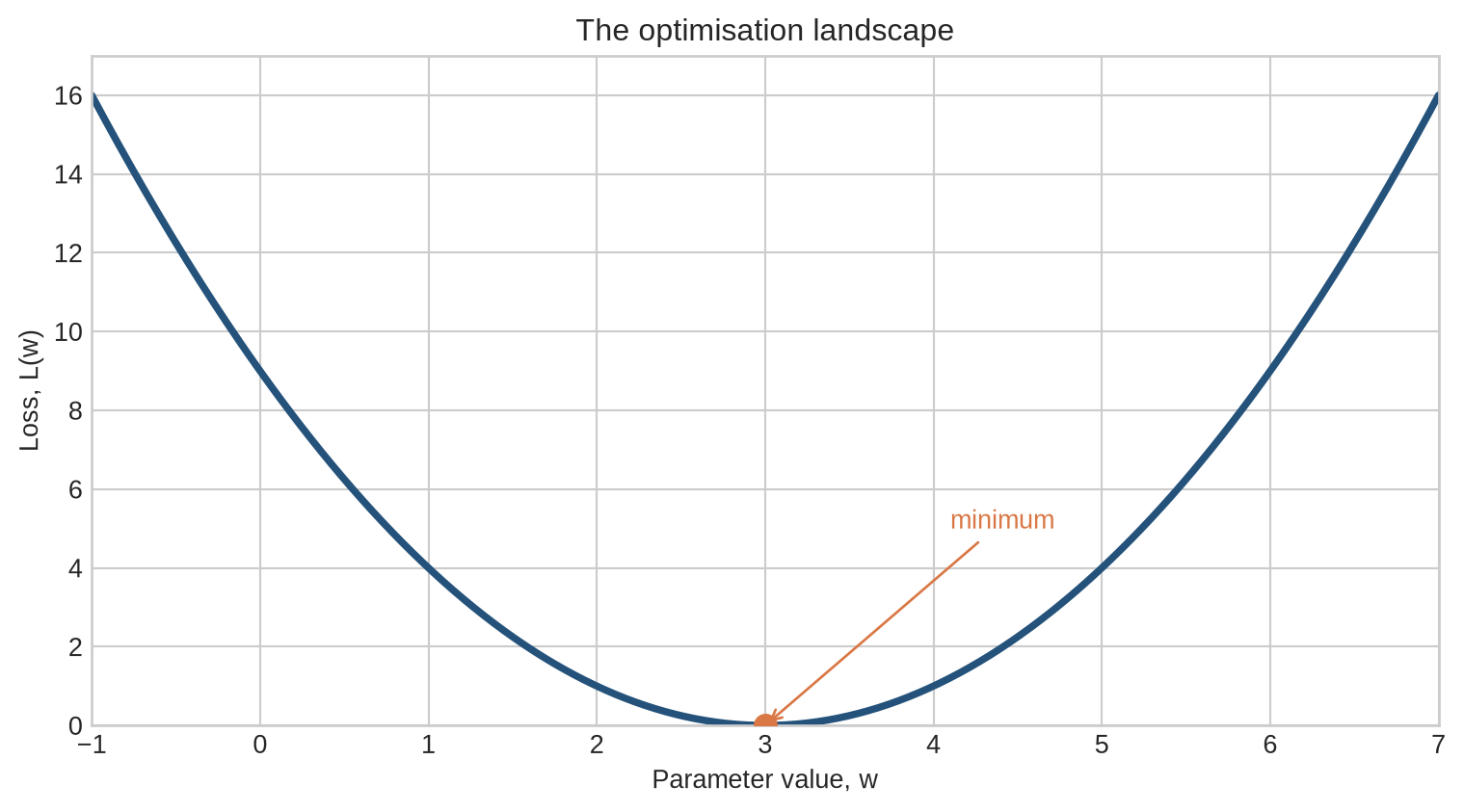
For this example, the best setting is $w=3$, because it makes the loss zero. Real models have far more settings and much more complicated loss functions, but one setting is enough to see the basic problem: we are at one value of $w$ and need a principled way to choose the next value.
The chart shows every possible setting for this small example. Along the bottom is the current value of $w$; the height of the curve is the loss produced by that value. The orange point is the lowest point on the curve. A real training procedure cannot usually draw this whole chart, but it can still use information from the part of the curve immediately around its current setting.
```{python}
#| label: fig-loss-curve
#| fig-cap: "A simple loss function. The training objective is to move toward the minimum at w = 3."
#| fig-alt: "A U-shaped loss curve with its minimum marked at w equals 3."
import numpy as np
import matplotlib.pyplot as plt

plt.style.use("seaborn-v0_8-whitegrid")
blue, teal, orange = "#24527a", "#3a9188", "#d97745"

w_values = np.linspace(-1, 7, 400)
loss_values = (w_values - 3) ** 2

fig, ax = plt.subplots(figsize=(8, 4.5))
ax.plot(w_values, loss_values, color=blue, linewidth=2.8)
ax.scatter([3], [0], color=orange, s=70, zorder=3)
ax.annotate("minimum", xy=(3, 0), xytext=(4.1, 5),
            arrowprops={"arrowstyle": "->", "color": orange}, color=orange)
ax.set_xlabel("Parameter value, w")
ax.set_ylabel("Loss, L(w)")
ax.set_title("The optimisation landscape")
ax.set_xlim(-1, 7)
ax.set_ylim(0, 17)
plt.tight_layout()
plt.show()
```
The curve is often called a loss landscape. It is simply a picture of the score attached to each possible setting of $w$. Training means changing the setting so that the score falls.
## Level 1 - Intuition
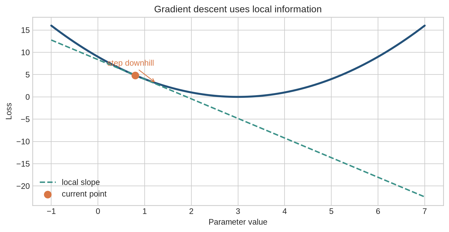
Suppose the rule currently uses $w=0.8$, marked by the orange point in the next figure. The programme does not know the full curve in a real model, but it can ask a local question: if $w$ were made slightly larger, would the loss go up or down? That is enough information to decide the direction of the next change.
```{python}
#| label: fig-intuitive-slope
#| fig-cap: "The local slope indicates which direction lowers the loss."
#| fig-alt: "A U-shaped loss curve with a current point, a tangent line, and a downward step toward the minimum."
current_w = 0.8
current_loss = (current_w - 3) ** 2
tangent = current_loss + 2 * (current_w - 3) * (w_values - current_w)
fig, ax = plt.subplots(figsize=(8, 4.2))
ax.plot(w_values, loss_values, color=blue, linewidth=2.5)
ax.plot(w_values, tangent, color=teal, linestyle="--", linewidth=1.8, label="local slope")
ax.scatter([current_w], [current_loss], color=orange, s=75, zorder=3, label="current point")
ax.annotate("step downhill", xy=(1.25, (1.25 - 3) ** 2), xytext=(0.2, 7),
            arrowprops={"arrowstyle": "->", "color": orange}, color=orange)
ax.set(xlabel="Parameter value", ylabel="Loss", title="Gradient descent uses local information")
ax.legend(frameon=False)
plt.tight_layout()
plt.show()
```
The solid curve shows the loss for every setting in this toy example. The dashed line touches the curve at the current point and shows its local tilt. Here it slopes downward to the right, so a slightly larger value of $w$ should reduce the loss. The update follows this local tilt; it does not rely on knowing that the orange minimum lies at $w=3$.
The local tilt is called the **gradient**. In a one-setting problem, it tells us whether to increase or decrease the setting. In a many-setting problem, it gives one such direction for each setting. Gradient descent is the repeated process of calculating these directions, changing the settings a little, and calculating them again.
::: {.concept-box .concept-core #concept-gradient-descent data-term="Gradient descent" data-domain="Foundations" data-symbols="gradient; learning rate"}
**Gradient descent.** A procedure for improving a fitted rule step by step. The **gradient** indicates how a small change in each parameter would change the loss, and the **learning rate** determines the size of the step.
:::
### Why not make one enormous step?
If the loss falls when $w$ increases, it does not follow that the largest possible increase is best. A very large change can pass the low point and land where the loss is high again. The **learning rate** controls the size of each change.
- A very small learning rate produces careful but slow progress.
- A suitable learning rate produces stable progress.
- A very large learning rate can cause the model to jump back and forth or diverge.
The aim is not to make the parameter move as far as possible. It is to reduce loss reliably over a sequence of updates. Level 2 follows one complete update: make predictions, calculate loss, calculate the gradient, and change the parameters.
## Level 2 - Mechanics
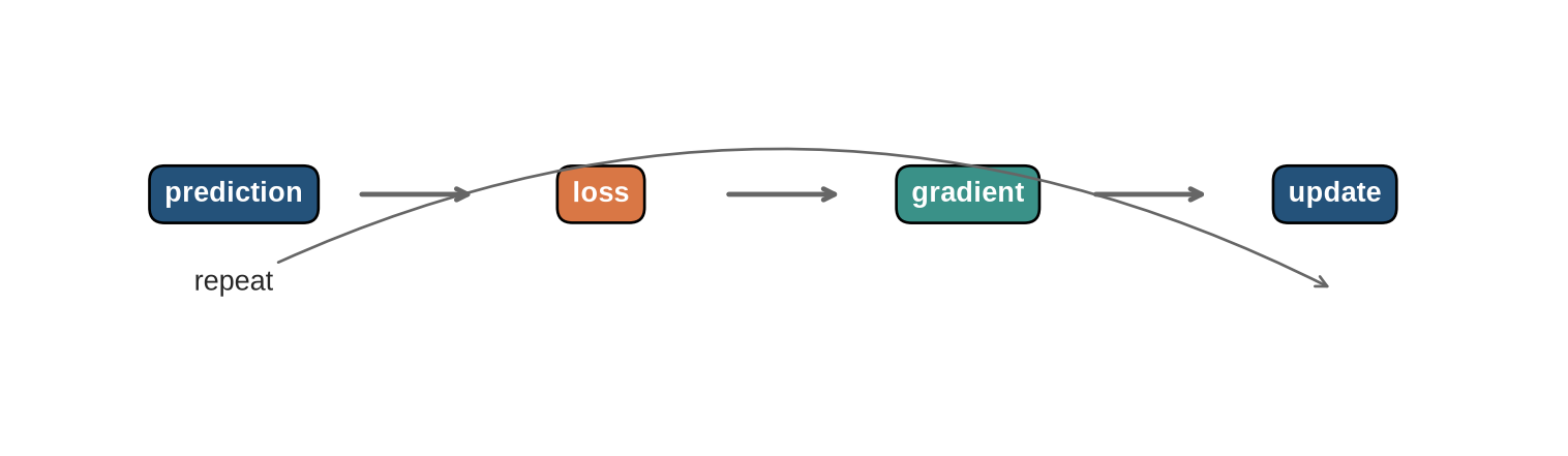
One update has four linked stages. The model first makes predictions using its current settings. Those predictions are scored against the recorded outcomes. The gradient then shows how the score would respond to small changes in the settings, and the update applies one chosen change. The diagram gives the order; each stage uses the result of the preceding one.
```{python}
#| label: fig-learning-cycle
#| fig-cap: "One learning step repeats prediction, loss calculation, gradient calculation, and parameter update."
#| fig-alt: "A circular four-step diagram showing prediction, loss, gradient, and update."
fig, ax = plt.subplots(figsize=(8, 2.4))
labels = [(0.14, "prediction", blue), (0.38, "loss", orange), (0.62, "gradient", teal), (0.86, "update", blue)]
for xpos, label, colour in labels:
    ax.text(xpos, 0.58, label, ha="center", va="center", color="white", weight="bold",
            bbox={"boxstyle": "round,pad=0.55", "facecolor": colour})
for left, right in zip(labels[:-1], labels[1:]):
    ax.annotate("", xy=(right[0] - 0.08, 0.58), xytext=(left[0] + 0.08, 0.58),
                arrowprops={"arrowstyle": "->", "lw": 1.8, "color": "#666666"})
ax.annotate("repeat", xy=(0.86, 0.35), xytext=(0.14, 0.35),
            arrowprops={"arrowstyle": "->", "connectionstyle": "arc3,rad=-0.25", "color": "#666666"}, ha="center")
ax.set_xlim(0, 1); ax.set_ylim(0, 1); ax.axis("off")
plt.tight_layout()
plt.show()
```
The diagram makes clear that loss comes before the gradient. The model cannot calculate a direction for improvement until it has first made predictions and scored them. After the update, the changed settings produce new predictions, and the cycle begins again.
### The learning cycle
The loss is feedback, not an instruction. A loss of 42 tells us that the model is wrong, but it does not itself identify the parameter that should change or the direction of the change. The gradient provides that information.
### A concrete prediction problem
Suppose the programme-uptake model predicts a continuous uptake score from one feature, such as distance to a service point. A simple model is:
$$
\hat{y}=wx+b,
$$
where $x$ is distance, $w$ is the learned slope, and $b$ is the learned intercept. For a collection of households, the model produces predictions $\hat{y}_1,\ldots,\hat{y}_n$. A common loss is the mean squared error:
$$
L(w,b)=\frac{1}{n}\sum_{i=1}^n(\hat{y}_i-y_i)^2.
$$
The model does not “know” that a particular prediction is too high in the human sense. The loss converts the difference between prediction and target into a number that can be differentiated. Gradient descent then changes $w$ and $b$ together.
### What a slope means locally
Near its current value, the slope tells the model whether a small increase in $w$ is expected to raise or lower the loss. A positive slope means that increasing $w$ makes the loss worse, so the update moves downward. A negative slope means that increasing $w$ improves the loss, so the update moves upward. The size of the slope helps determine how strongly the algorithm responds.
### What happens at a minimum?
At the bottom of a smooth valley, the local slope is zero because neither small direction lowers the loss immediately. The quadratic example has one such lowest point. Large neural-network objectives have a more complicated shape; Level 4 returns to what that changes in practice.
### One parameter at a time
In the running example, start at $w=0$. The loss is:
$$
L(0)=(0-3)^2=9.
$$
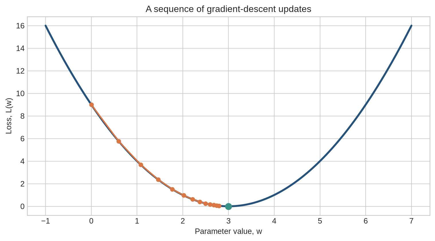
The curve slopes downward as $w$ increases, so a sensible update should increase $w$. After several updates, $w$ should approach 3.
The points in the figure are the actual parameter values after successive updates. Their vertical positions are the corresponding losses. The points move closer together as they approach the minimum because the derivative becomes smaller. This is the behaviour that the update equation must produce in this example.
```{python}
#| label: fig-optimisation-path
#| fig-cap: "Gradient descent takes a sequence of small steps toward the minimum."
#| fig-alt: "A loss curve with a series of connected points moving from w equals 0 toward w equals 3."
w_values = np.linspace(-1, 7, 400)
loss_values = (w_values - 3) ** 2

w = 0.0
learning_rate = 0.1
history = [w]

for _ in range(12):
    gradient = 2 * (w - 3)
    w = w - learning_rate * gradient
    history.append(w)

fig, ax = plt.subplots(figsize=(8, 4.5))
ax.plot(w_values, loss_values, color=blue, linewidth=2.5)
ax.plot(history, [(value - 3) ** 2 for value in history],
        marker="o", color=orange, linewidth=1.8, markersize=5)
ax.scatter([3], [0], color=teal, s=65, zorder=3)
ax.set_xlabel("Parameter value, w")
ax.set_ylabel("Loss, L(w)")
ax.set_title("A sequence of gradient-descent updates")
plt.tight_layout()
plt.show()
```
The worked update identifies the two ingredients that must be calculated at every step: a local direction and a step size. The mathematics below gives that direction a precise name—the gradient—and shows why the update subtracts it.
## Level 3 - Mathematics & Code
Level 2 established the order of one update. This level writes the same calculation in notation, derives the local direction, and implements the update so that each line of code can be checked against the equation.
### What is a gradient?
For a single parameter, the gradient is just the derivative:
$$
\frac{dL}{dw}.
$$
For the running example:
$$
L(w)=(w-3)^2,
\qquad
\frac{dL}{dw}=2(w-3).
$$
The derivative has two parts. The factor 2 comes from differentiating the square. The term $(w-3)$ records how far the current parameter is from the value that minimises the loss. At $w=3$, the derivative is zero. At values below 3 it is negative; at values above 3 it is positive.
At $w=0$, the derivative is $-6$. The negative sign means that increasing $w$ would reduce the loss. Gradient descent moves in the opposite direction of the derivative:
$$
w_{\mathrm{new}} = w_{\mathrm{old}} - \eta\frac{dL}{dw}.
$$
With $w=0$ and $\eta=0.1$:
$$
w_{\mathrm{new}}=0-0.1(-6)=0.6.
$$
The parameter moves toward the minimum.
The calculation illustrates the role of the minus sign. At $w=0$, the derivative is negative, so subtracting it increases the parameter. The learning rate scales the change: without $\eta$, the update would be fixed at six units, which would be unnecessarily large for this example. The update uses the derivative to choose a direction and the learning rate to choose a distance.
### A full worked update
Let $w_0=0$ and $\eta=0.1$. The first three iterations are:
| Step | $w_t$ | $L(w_t)$ | $dL/dw$ | $w_{t+1}$ |
|---:|---:|---:|---:|---:|
| 0 | 0.000 | 9.000 | -6.000 | 0.600 |
| 1 | 0.600 | 5.760 | -4.800 | 1.080 |
| 2 | 1.080 | 3.686 | -3.840 | 1.464 |
The updates become smaller as $w$ approaches 3 because the derivative approaches zero. For this particular quadratic, the recurrence can be written directly:
$$
w_{t+1}=w_t-2\eta(w_t-3).
$$
Rearranging around the optimum gives:
$$
w_{t+1}-3=(1-2\eta)(w_t-3).
$$
This equation makes the learning-rate constraint visible. For $0<\eta<1$, the distance from the optimum shrinks in magnitude. When $\eta=1$, the next step jumps across the optimum by the same distance. When $\eta>1$, the distance grows and the algorithm diverges for this example.
### Two parameters and a contour plot
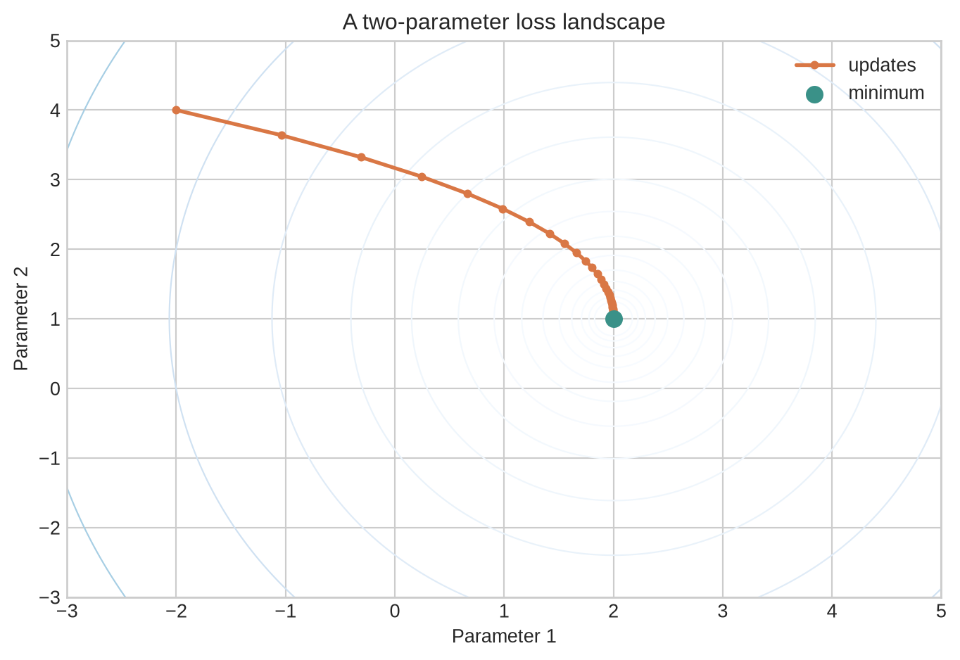
With two parameters, the loss is a surface rather than a curve. A contour plot shows equal-loss lines from above. The gradient points perpendicular to the contour passing through the current point, toward the direction of steepest increase. The update travels in the opposite direction.
```{python}
#| label: fig-contour-path
#| fig-cap: "In two dimensions, the gradient-descent path crosses contours toward lower loss."
#| fig-alt: "A contour plot of a tilted quadratic surface with an orange optimisation path moving toward its minimum."
u = np.linspace(-3, 5, 250)
v = np.linspace(-3, 5, 250)
U, V = np.meshgrid(u, v)
surface = (U - 2) ** 2 + 0.5 * (V - 1) ** 2

point = np.array([-2.0, 4.0])
path = [point.copy()]
for _ in range(28):
    grad = np.array([2 * (point[0] - 2), (point[1] - 1)])
    point = point - 0.12 * grad
    path.append(point.copy())
path = np.array(path)

fig, ax = plt.subplots(figsize=(7.2, 5))
levels = np.geomspace(0.03, 80, 16)
ax.contour(U, V, surface, levels=levels, cmap="Blues", linewidths=0.8)
ax.plot(path[:, 0], path[:, 1], color=orange, marker="o", markersize=3.5,
        linewidth=2, label="updates")
ax.scatter([2], [1], color=teal, s=70, label="minimum", zorder=3)
ax.set(xlabel="Parameter 1", ylabel="Parameter 2", title="A two-parameter loss landscape")
ax.legend(frameon=False)
plt.tight_layout()
plt.show()
```
Each contour represents a set of parameter combinations with the same loss. The orange path records successive updates, while the teal point marks the minimum of this constructed surface. In more complicated models the contours are not usually ellipses, but the local rule is the same: calculate the gradient at the current point and move in the opposite direction.
### Finite differences: a useful diagnostic
Before trusting an automatic derivative, it is useful to understand numerical differentiation. A centred finite-difference estimate is:
$$
\frac{dL}{dw}\approx\frac{L(w+h)-L(w-h)}{2h}.
$$
```{python}
w = 1.2
h = 1e-5
analytic = 2 * (w - 3)
finite_difference = (((w + h) - 3) ** 2 - ((w - h) - 3) ** 2) / (2 * h)
print(f"analytic derivative:        {analytic:.6f}")
print(f"finite-difference estimate:  {finite_difference:.6f}")
```
Finite differences are slow for a model with millions of parameters and can become inaccurate when $h$ is too small. Automatic differentiation uses the computational structure of the model to calculate exact derivatives up to floating-point precision, which is why it is preferred in training frameworks.
The finite-difference calculation is useful because it checks the derivative without relying on the derivative formula used in the training code. If the analytic and numerical values disagree substantially, the problem may be in the model, the loss, the implementation, or the choice of step size $h$. A gradient check is therefore a debugging tool, not an alternative optimiser.
### From one parameter to many
Real models have a parameter vector $\theta$ rather than a single $w$. Let $d$ denote the number of parameters:
$$
\theta = (\theta_1, \theta_2, \ldots, \theta_d).
$$
The gradient is a vector of partial derivatives:
$$
\nabla_\theta L =
\left(
\frac{\partial L}{\partial \theta_1},
\frac{\partial L}{\partial \theta_2},
\ldots,
\frac{\partial L}{\partial \theta_d}
\right).
$$
Every parameter receives its own directional signal. The update is:
$$
\theta_{\mathrm{new}} = \theta_{\mathrm{old}} - \eta\nabla_\theta L.
$$
### NumPy implementation
The following implementation makes the update explicit. It does not use automatic differentiation, so the derivative is written by hand.
```{python}
#| label: fig-learning-curve
#| fig-cap: "The parameter approaches the optimum while the loss falls."
#| fig-alt: "Two panels showing parameter value approaching 3 and loss approaching zero over training steps."
w = 0.0
learning_rate = 0.1
weights, losses = [], []

for step in range(25):
    loss = (w - 3) ** 2
    gradient = 2 * (w - 3)
    weights.append(w)
    losses.append(loss)
    w -= learning_rate * gradient

fig, axes = plt.subplots(1, 2, figsize=(9, 3.7))
axes[0].plot(weights, color=teal, linewidth=2.5)
axes[0].axhline(3, color=orange, linestyle="--", label="optimum")
axes[0].set(xlabel="Step", ylabel="w", title="Parameter")
axes[0].legend(frameon=False)
axes[1].plot(losses, color=blue, linewidth=2.5)
axes[1].set(xlabel="Step", ylabel="Loss", title="Objective")
plt.tight_layout()
plt.show()
```
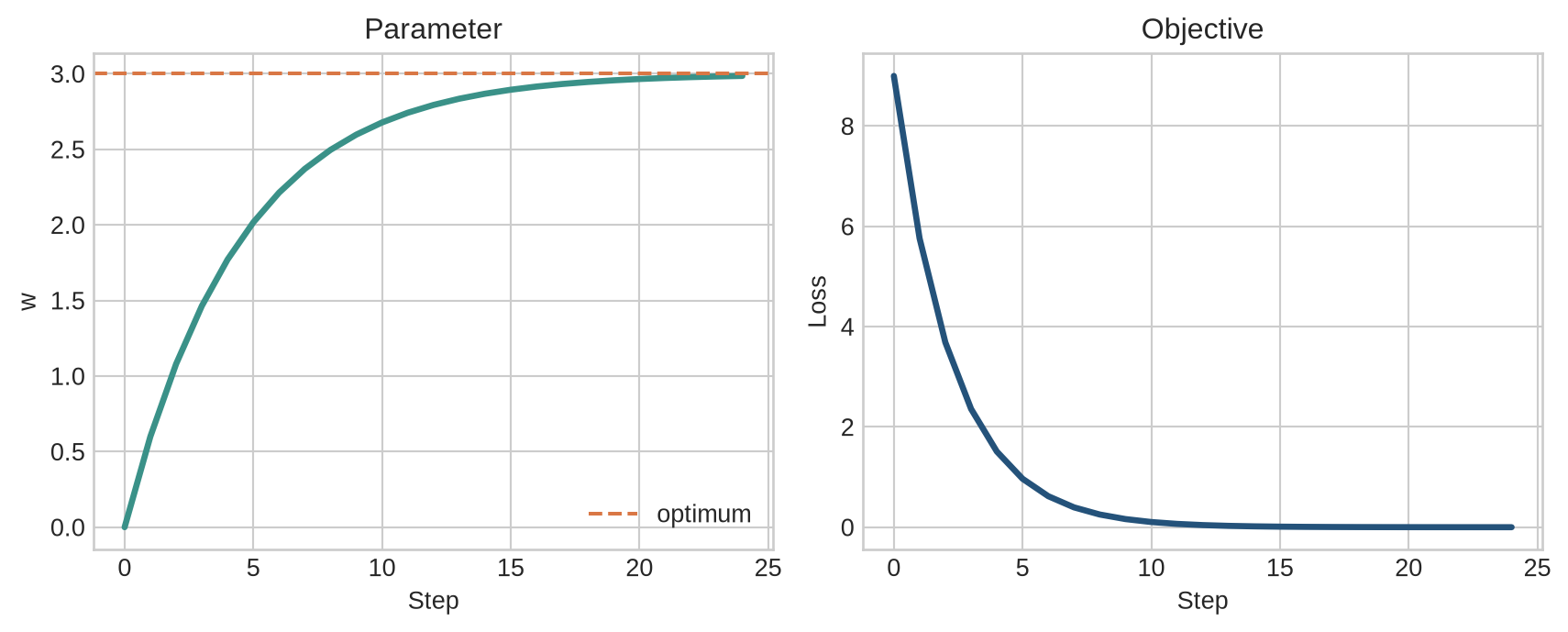
The loop follows the update rule directly. It evaluates the current loss, calculates the derivative at the current parameter, and then overwrites $w$ with the updated value. Recording the parameter and loss histories makes the learning process observable; the final value alone would not show how the algorithm reached its result.
### PyTorch implementation
In practice, frameworks calculate derivatives automatically. The following code uses PyTorch's computation graph and automatic differentiation.
```{python}
import torch

w = torch.tensor(0.0, requires_grad=True)
learning_rate = 0.1

for step in range(25):
    loss = (w - 3) ** 2
    loss.backward()

    with torch.no_grad():
        w -= learning_rate * w.grad
        w.grad.zero_()

print(f"final parameter: {w.item():.3f}")
print(f"final loss: {(w.item() - 3) ** 2:.6f}")
```
There are two distinct operations here:
- `loss.backward()` computes the gradient;
- the subtraction inside `torch.no_grad()` applies the update.
This distinction becomes important in [Chapter 4](04-backpropagation.qmd), which examines backpropagation.
The PyTorch loop produces the same parameter trajectory as the hand-written NumPy loop, but the derivative is obtained from the computation graph. `requires_grad=True` asks PyTorch to track operations involving `w`; `loss.backward()` computes the derivative; and the `torch.no_grad()` block applies the update without adding the update itself to the graph. Clearing `w.grad` matters because PyTorch accumulates gradients by default.
### Learning rates and failure modes
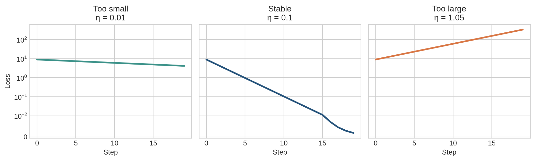
The learning rate is not a minor implementation detail. It changes the path through the landscape.
```{python}
#| label: fig-learning-rates
#| fig-cap: "Different learning rates produce different optimisation behaviour."
#| fig-alt: "Three loss curves over training steps, showing slow, stable, and unstable learning rates."
rates = [0.01, 0.1, 1.05]
labels = ["Too small", "Stable", "Too large"]
colors = [teal, blue, orange]

fig, axes = plt.subplots(1, 3, figsize=(11, 3.4), sharey=True)
for ax, rate, label, color in zip(axes, rates, labels, colors):
    w = 0.0
    values = []
    for _ in range(20):
        values.append((w - 3) ** 2)
        w -= rate * 2 * (w - 3)
    ax.plot(values, color=color, linewidth=2.4)
    ax.set_title(f"{label}\nη = {rate}")
    ax.set_xlabel("Step")
    ax.set_yscale("symlog", linthresh=0.01)
axes[0].set_ylabel("Loss")
plt.tight_layout()
plt.show()
```
When the rate is too small, the algorithm is stable but inefficient. When it is too large, the update can overshoot the minimum repeatedly. Real training often changes the learning rate over time, using warm-up, decay, or schedules adapted to the model and batch size.
## Level 4 - Research & Systems
The one-parameter example makes the update easy to see, but it hides the conditions that determine whether optimisation is practical. At this level, the relevant objects are noisy gradients, mini-batches, adaptive optimiser state, memory, communication, and the changing geometry of large neural-network objectives.
### Batch and stochastic updates
Suppose the training dataset contains one million examples. Computing the exact gradient over all of them before every update would be expensive. Instead, modern training usually uses a mini-batch such as 256 examples.
- **Batch gradient descent** uses the complete dataset for each update.
- **Stochastic gradient descent** uses one example at a time.
- **Mini-batch gradient descent** uses a small random subset and is the standard practical compromise.
Mini-batches make updates noisy because different samples produce different gradient estimates. This noise changes the optimisation path and can sometimes help the optimiser leave poorly performing regions, although it does not guarantee a better solution. Mini-batches also map naturally onto parallel hardware.
The stochastic-gradient perspective has a long history. Robbins and Monro formalised stochastic approximation in 1951, and stochastic-gradient methods became central to large-scale learning because they replace an expensive full-dataset gradient with an estimate based on sampled data [@robbins1951]. Bottou, Curtis, and Nocedal explain why this setting differs from classical numerical optimisation: the objective is high-dimensional, the gradients are noisy, and each update must be cheap enough to perform many times [@bottou2018].
For a mini-batch $B_t$, the update uses:
$$
g_t=\frac{1}{|B_t|}\sum_{i\in B_t}\nabla_\theta\ell_i(\theta_t),
\qquad
\theta_{t+1}=\theta_t-\eta_tg_t.
$$
The mini-batch gradient is an estimator of the full gradient. Increasing the batch size usually reduces its variance, but it also increases the amount of data and memory required per update. The useful batch size is therefore a systems and statistical choice, not a universal constant.
The equation makes the source of the noise explicit: each update averages only the losses in $B_t$, not every example in the dataset. Two different mini-batches can therefore produce different gradients at the same parameter value. The optimiser must make progress despite this variation. Batch size changes both the cost of an update and the statistical information used to choose its direction.
### Adam and AdamW
SGD applies the same nominal learning rate to every parameter. Adam maintains moving averages of the gradient and the squared gradient. It uses these estimates to scale updates separately for different parameters. AdamW decouples weight decay from the adaptive gradient update, making the regularisation coefficient easier to interpret separately from the learning-rate adaptation.
These methods are still gradient descent in the broad sense: gradients provide the learning signal, and an optimiser converts that signal into parameter changes.
The distinction between SGD and Adam is therefore a distinction in how the same learning signal is processed. SGD uses the current gradient, possibly with momentum. Adam keeps additional state summarising recent gradients and rescales the current update. Those choices can change speed, stability, generalisation, and memory use; they do not change the fact that the model is being trained through parameter updates guided by derivatives.
Adam maintains exponentially decaying averages of the gradient and squared gradient [@kingma2014]:
$$
m_t=\beta_1m_{t-1}+(1-\beta_1)g_t,
$$
$$
v_t=\beta_2v_{t-1}+(1-\beta_2)g_t^2.
$$
After correcting the initial bias in these averages, Adam updates each parameter using a normalized first-moment estimate:
$$
\theta_{t+1}=\theta_t-\eta\frac{\hat m_t}{\sqrt{\hat v_t}+\epsilon}.
$$
The squared-gradient accumulator makes the effective step size coordinate-specific. This is particularly useful when different parameters receive gradients on very different scales.
AdamW separates weight decay from the adaptive gradient update. Loshchilov and Hutter show that ordinary L2 regularisation and weight decay are equivalent for plain SGD but not generally for adaptive methods; their decoupled formulation applies a direct shrinkage step [@adamw2019].
### The optimisation landscape of a neural network
The one-dimensional parabola is deliberately simple. A neural network's loss landscape has one dimension for every parameter. It can contain flat regions, steep ravines, saddle points, and many low-loss solutions. Visualisations of two-dimensional slices can help build intuition, but they should not be mistaken for a literal map of the full landscape.
At LLM scale, optimisation also involves:
- storing activations and gradients within GPU memory;
- communicating gradients across many accelerators;
- choosing numerical precision and loss-scaling strategies;
- balancing batch size, throughput, and generalisation;
- recovering from interrupted training through checkpoints.
### Why training is expensive
For a parameterised model, training requires at least a forward computation, storage of selected intermediate activations, a backward computation, and an optimiser update. In a distributed setting, workers must also exchange gradients or parameter updates. The time per step is therefore not determined only by the number of floating-point operations. It depends on memory bandwidth, communication topology, kernel efficiency, and whether the accelerator is kept busy.
This creates practical trade-offs:
- **Larger batches** improve hardware utilisation but may change optimisation dynamics.
- **Activation checkpointing** reduces memory use by recomputing parts of the forward pass.
- **Mixed precision** increases throughput and reduces memory use but requires numerical safeguards.
- **Gradient accumulation** simulates a larger batch when the device cannot hold it at once.
- **Learning-rate schedules** coordinate the optimisation regime with the changing scale of updates.
Comparisons between optimisers therefore need to specify the data, architecture, batch size, numerical precision, and hardware conditions under which the comparison was made.
### What the literature does and does not guarantee
For smooth convex objectives, gradient methods have clean convergence analyses. Deep-network training is generally non-convex, stochastic, and overparameterised. Empirical success therefore exceeds what simple textbook guarantees can explain. This does not make the equations useless; it means that theory, controlled experiments, and system measurements must be read together.
The update equation remains short. Making that equation reliable and affordable is a major part of modern ML engineering.
## Common misconceptions
### “The gradient tells the model the correct answer.”
No. The target and loss function define what counts as an error. The gradient tells us how small parameter changes would affect that error.
### “A zero gradient means the model is perfect.”
Not necessarily. A zero gradient can occur at a minimum, maximum, or saddle point. In numerical computation it can also result from saturation or underflow.
### “Gradient descent always finds the best possible model.”
There is generally no guarantee that a non-convex neural-network problem will reach a global optimum. In practice, the goal is usually a solution that performs well on unseen data.
### “More training steps always improve the model.”
Training loss may continue to fall while validation performance deteriorates. Optimisation and generalisation are related but distinct problems.
## Exercises
1. Explain the mountain analogy and identify the parameter, loss, gradient, and learning rate.
2. For $L(w)=(w-4)^2$, calculate the gradient at $w=1$.
3. Starting with $w=1$, use learning rate $0.1$ to perform two updates for $L(w)=(w-4)^2$.
4. Why is the gradient subtracted in the update rule?
5. Plot the optimisation path for learning rates $0.01$, $0.1$, and $1.05$. Describe what changes.
6. Why are mini-batches useful for both computation and optimisation?
7. Explain why a parameter can have a zero gradient even when the model is not useful.
8. Compare the roles of `loss.backward()` and `optimizer.step()`.
9. Why do large language models require checkpointing during training?
10. Write a short explanation of gradient descent for someone who knows algebra but has never studied machine learning.
11. For $L(w_1,w_2)=(w_1-2)^2+4(w_2+1)^2$, calculate the gradient at $(0,0)$ and make one update with learning rate $0.1$.
12. Two mini-batches produce gradients of $-1.0$ and $0.4$ for the same parameter. Explain why consecutive updates can move in different directions without making the optimisation procedure incoherent.
13. Run ten updates for $L(w)=(w-4)^2$ with learning rates $0.01$ and $0.4$. Compare their losses after the same number of updates.
14. A training loss becomes `NaN` after a large update. List two quantities you would inspect before reducing the learning rate and explain what each could show.
15. Explain why a plateau in the loss does not by itself identify whether the learning rate is too small, the gradient is zero, or the model is under-specified.
16. State which quantities must be saved to resume a stochastic gradient-descent run from the same next update, and distinguish them from the final model parameters.
## Summary
Gradient descent is a general method for reducing a loss by repeatedly moving parameters opposite the local gradient. The learning rate determines the size of each move. In real neural networks, gradients are estimated from mini-batches and transformed by optimisers such as SGD, Adam, and AdamW. At modern scale, the mathematics is only part of the challenge: memory, communication, precision, and throughput determine whether the optimisation process is practical.
## Looking ahead
Gradient descent tells us how parameters should change, but we have not yet explained how a network computes the gradient for every parameter efficiently. [Chapter 4](04-backpropagation.qmd) introduces backpropagation and the chain rule, which turn a forward computation into a complete set of gradients.
## Further reading
- Robbins and Monro, “A Stochastic Approximation Method,” the foundational paper on stochastic approximation [@robbins1951].
- Bottou, Curtis, and Nocedal, “Optimization Methods for Large-Scale Machine Learning,” a broad treatment of stochastic optimisation in ML [@bottou2018].
- Kingma and Ba, “Adam: A Method for Stochastic Optimization,” the original Adam paper [@kingma2014].
- Loshchilov and Hutter, “Decoupled Weight Decay Regularization,” the AdamW paper [@adamw2019].