---
title: "Normalisation"
subtitle: "Choosing the values that define a reference scale"
---
## The problem
Chapter 11 chose initial weights so that the first forward and backward pass could work. After training begins, updates change the values reaching later layers. A layer may then receive values with a different offset or spread from one batch to the next, even though its own parameters have not changed.
Normalisation gives those values a reference scale. The arithmetic is simple: compare a value with a selected set of values, then recalculate it relative to that set. The consequential choice is which values belong in the reference. That choice determines whether one observation can affect another and whether the same rule can be used during training and evaluation.
### A visible reference choice
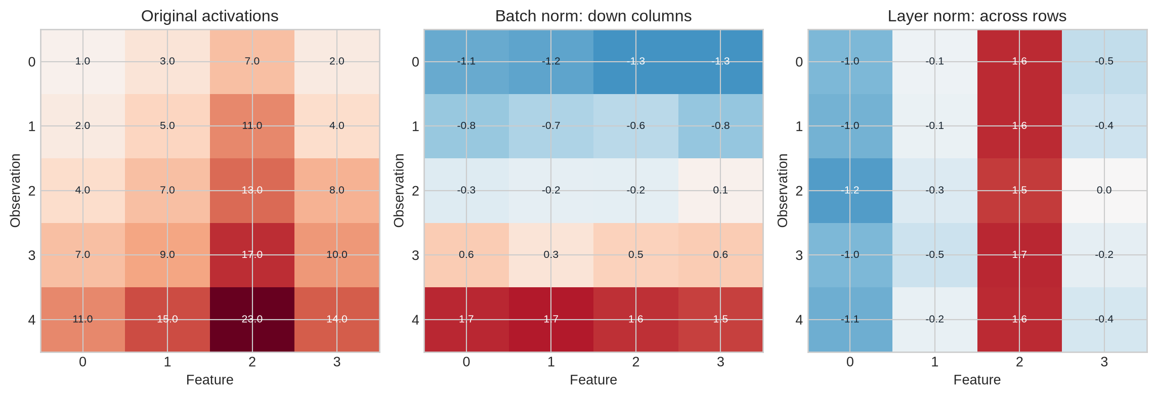
The chapter begins with a matrix containing five observations and four features. Its rows have different overall levels, while its columns have different scales. This makes the choice of normalisation axis visible.
Read the three heatmaps by following a single value across panels. In the batch-normalised panel, its comparison group is the other entries in the same column. In the layer-normalised panel, its comparison group is the other entries in the same row. The transformed values differ because the question asked of them differs.
```{python}
#| label: fig-normalisation-axes
#| fig-cap: "Batch and layer normalisation use different reference sets, even when applied to the same activation matrix."
#| fig-alt: "Three annotated heatmaps show an original activation matrix, the same matrix normalised down each feature across observations, and the matrix normalised across features within each observation."
import numpy as np
import matplotlib.pyplot as plt

plt.style.use("seaborn-v0_8-whitegrid")
blue, teal, orange, purple, grey = "#24527a", "#3a9188", "#d97745", "#7a5195", "#5f6b76"

X = np.array([
    [ 1.0,  3.0,  7.0,  2.0],
    [ 2.0,  5.0, 11.0,  4.0],
    [ 4.0,  7.0, 13.0,  8.0],
    [ 7.0,  9.0, 17.0, 10.0],
    [11.0, 15.0, 23.0, 14.0],
])

def standardise(x, axis, eps=1e-5):
    mean = x.mean(axis=axis, keepdims=True)
    variance = x.var(axis=axis, keepdims=True)
    return (x - mean) / np.sqrt(variance + eps)

X_batch = standardise(X, axis=0)  # each feature uses all observations
X_layer = standardise(X, axis=1)  # each observation uses all features

fig, axes = plt.subplots(1, 3, figsize=(12, 4.2))
panels = [(X, "Original activations"),
          (X_batch, "Batch norm: down columns"),
          (X_layer, "Layer norm: across rows")]
for ax, (values, title) in zip(axes, panels):
    limit = max(2.2, np.abs(values).max())
    image = ax.imshow(values, cmap="RdBu_r", aspect="auto", vmin=-limit, vmax=limit)
    for i in range(values.shape[0]):
        for j in range(values.shape[1]):
            ax.text(j, i, f"{values[i,j]:.1f}", ha="center", va="center", fontsize=8,
                    color="white" if abs(values[i,j]) > 0.55 * limit else "#18242f")
    ax.set_title(title); ax.set_xlabel("Feature"); ax.set_xticks(range(4))
    ax.set_ylabel("Observation"); ax.set_yticks(range(5))
plt.tight_layout(); plt.show()
```
The two normalised matrices are not competing calculations of the same quantity. Batch normalisation asks where a feature value lies relative to that feature in other observations. Layer normalisation asks where a feature lies relative to the other features in the same observation. The appropriate question depends on the architecture and on which observations should influence one another.
::: {.concept-box .concept-core #concept-normalisation data-term="Normalisation" data-domain="Training and evaluation"}
**Normalisation.** A transformation that expresses values relative to a selected reference set. The reference can be a batch, one observation, a channel group, or a vector; that choice determines which values influence one another and how training differs from inference.
:::
## Level 1 - Intuition
### A value needs a reference
A value of $30$ has little meaning without its unit and a comparison range. A value two standard deviations above a relevant mean tells us more because it supplies a reference. Normalisation does the same for model activations: it describes a value relative to selected other values.
This transformation does not make every activation uninformative or identical. It removes selected location and scale information, then retains the pattern of relative deviations. A value above its reference mean remains positive; a value below it remains negative. Learned scale and shift parameters can subsequently restore a useful magnitude and offset.
### The reference set determines the meaning
In the running matrix, batch normalisation treats each column as a feature. The value $23$ in the final row is compared with the other values in its column: $7$, $11$, $13$, and $17$. Layer normalisation instead compares $23$ with $11$, $15$, and $14$ in the same row. Its normalised value therefore answers a different question.
This distinction also identifies a dependency. Under batch normalisation, changing one observation can alter the normalised outputs of other observations in the mini-batch. Under layer normalisation, changing one observation does not change another observation's result. That independence is important for variable batch sizes and sequence models.
### Centring and scaling do different jobs
Subtracting a mean recentres values around zero. Dividing by a standard deviation expresses them in units of spread. RMS normalisation performs the second operation without the first: it controls vector magnitude while retaining information in the mean. Normalisation is therefore not one indivisible recipe.
```{python}
#| label: fig-normalisation-vector
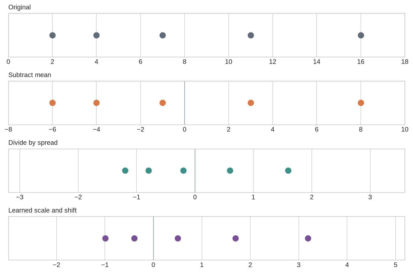
#| fig-cap: "Centring changes the offset, scaling changes the spread, and a learned affine transformation sets a new working range."
#| fig-alt: "Four aligned dot plots show an original vector, its centred values, its standardised values, and values after a learned scale and shift."
vector = np.array([2.0, 4.0, 7.0, 11.0, 16.0])
centred = vector - vector.mean()
normalised = centred / vector.std()
gamma, beta = 1.5, 0.8
affine = gamma * normalised + beta

fig, axes = plt.subplots(4, 1, figsize=(9, 6), sharex=False)
for ax, values, title, colour in zip(
    axes, [vector, centred, normalised, affine],
    ["Original", "Subtract mean", "Divide by spread", "Learned scale and shift"],
    [grey, orange, teal, purple]):
    ax.scatter(values, np.zeros_like(values), s=75, color=colour, zorder=3)
    ax.axvline(0, color="#9aa5ad", linewidth=1); ax.set_yticks([]); ax.set_title(title, loc="left", fontsize=10)
    ax.set_xlim(values.min()-2, values.max()+2)
plt.tight_layout(); plt.show()
```
The standardised vector has mean zero and variance close to one. The final transformation no longer has those exact statistics because $γ=1.5$ and $β=0.8$. This is intentional. Normalisation provides a controlled reference frame; it does not force every layer to remain permanently standard normal.
Once the reference is specified, the implementation must calculate its statistics, decide when they are reused, and preserve the dependencies that choice implies. Level 2 follows these operations for batch, layer, group, and RMS normalisation.
## Level 2 - Mechanics
### A normalisation layer performs three operations
First, the layer selects a set of values and calculates a statistic from them. For standard batch or layer normalisation, these statistics are a mean and variance. Second, it subtracts the mean and divides by the square root of the variance plus a small constant. Third, it applies learned scale and shift parameters, conventionally called gamma ($γ$) and beta ($β$).
The small constant epsilon prevents division by zero when a reference set has little or no variation. Gamma and beta give the model control over the resulting coordinate system. Without them, every normalised channel would be constrained to a fixed location and scale even when the task benefits from another range.
### Batch normalisation has separate training and evaluation mechanics
During training, batch normalisation calculates statistics from the current mini-batch. It also updates running estimates of the feature means and variances. During evaluation, it uses those stored estimates rather than allowing the composition of a test batch to change a prediction. Calling the model's training or evaluation mode is therefore part of the mathematical behaviour, not an administrative detail.
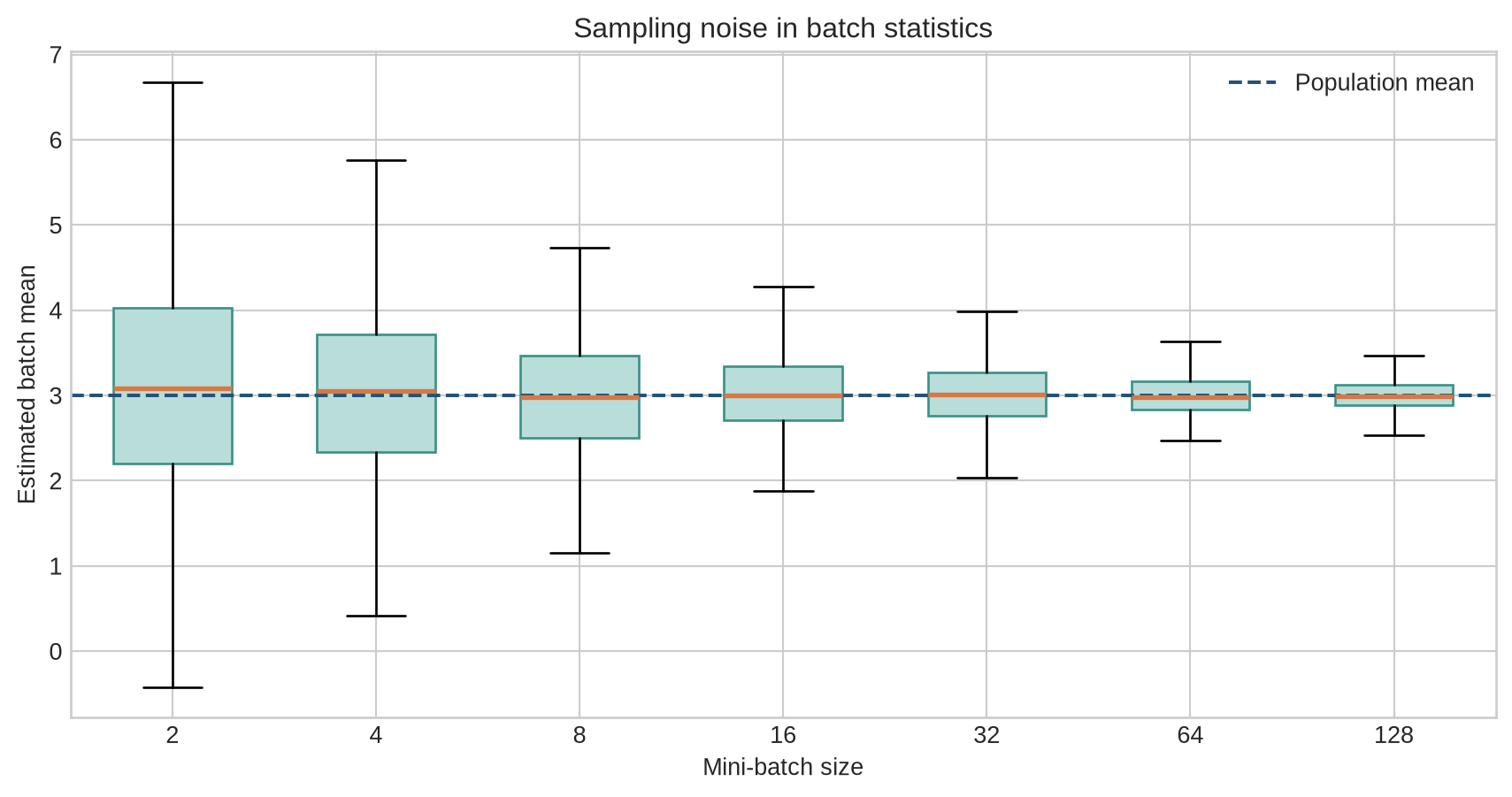
Small batches estimate population statistics noisily. The following simulation draws repeated mini-batches from the same population. Every dot is a valid batch mean, yet the range is much wider for two observations than for 128.
```{python}
#| label: fig-batch-size-noise
#| fig-cap: "Small mini-batches produce noisier estimates of the same population mean."
#| fig-alt: "Box plots show wide distributions of estimated means at batch sizes two and four, narrowing progressively through batch size 128 around the true mean of three."
rng = np.random.default_rng(124)
batch_sizes = [2, 4, 8, 16, 32, 64, 128]
estimates = [rng.normal(3, 2, size=(600, size)).mean(axis=1) for size in batch_sizes]
fig, ax = plt.subplots(figsize=(9, 4.8))
parts = ax.boxplot(estimates, positions=np.arange(len(batch_sizes)), widths=0.58,
                   patch_artist=True, showfliers=False)
for box in parts["boxes"]: box.set(facecolor="#b9ddd8", edgecolor=teal)
for median in parts["medians"]: median.set(color=orange, linewidth=2)
ax.axhline(3, color=blue, linestyle="--", label="Population mean")
ax.set_xticks(np.arange(len(batch_sizes)), batch_sizes)
ax.set_xlabel("Mini-batch size"); ax.set_ylabel("Estimated batch mean")
ax.set_title("Sampling noise in batch statistics"); ax.legend()
plt.tight_layout(); plt.show()
```
The noise can have a regularising effect, but it also makes behaviour depend on batch construction. When memory constraints force very small batches, batch normalisation can become unreliable.
### Evaluation uses the training reference distribution
```{python}
#| label: fig-batchnorm-train-eval
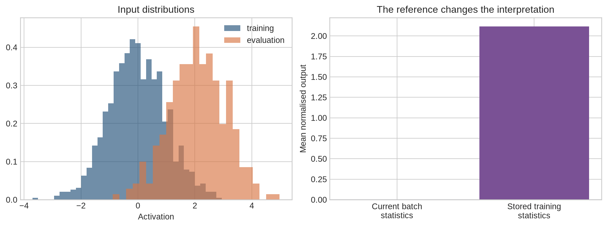
#| fig-cap: "Batch statistics centre each current batch, while stored training statistics expose a shifted evaluation distribution."
#| fig-alt: "A two-panel figure shows training and shifted evaluation value distributions, followed by bars comparing their output means under current-batch and stored-statistic normalisation."
rng = np.random.default_rng(90)
train = rng.normal(0, 1, 1000)
evaluation = rng.normal(2, 1, 300)
train_mean, train_var = train.mean(), train.var()
current_batch_output = (evaluation - evaluation.mean()) / np.sqrt(evaluation.var() + 1e-5)
stored_output = (evaluation - train_mean) / np.sqrt(train_var + 1e-5)

fig, axes = plt.subplots(1, 2, figsize=(10.5, 4))
axes[0].hist(train, bins=35, density=True, alpha=.65, color=blue, label="training")
axes[0].hist(evaluation, bins=25, density=True, alpha=.65, color=orange, label="evaluation")
axes[0].set_title("Input distributions"); axes[0].set_xlabel("Activation"); axes[0].legend()
axes[1].bar(["Current batch\nstatistics", "Stored training\nstatistics"],
            [current_batch_output.mean(), stored_output.mean()], color=[teal, purple])
axes[1].axhline(0, color=grey, linewidth=1); axes[1].set_ylabel("Mean normalised output")
axes[1].set_title("The reference changes the interpretation")
plt.tight_layout(); plt.show()
```
Using current evaluation-batch statistics would hide the mean shift and make one prediction depend on whichever other cases happen to be evaluated with it. Stored training statistics preserve a stable function. The non-zero output under stored statistics is not a bug: it signals that evaluation activations differ from the training reference.
### Layer, group, and RMS normalisation avoid batch dependence
Layer normalisation calculates statistics across the feature dimensions of one observation or token [@ba2016layernorm]. Group normalisation divides channels within one observation into groups and normalises each group [@wu2018groupnorm]. RMS normalisation divides by the root mean square within a vector but does not subtract its mean [@zhang2019rmsnorm]. None requires running batch statistics.
::: {.concept-box .concept-distinction #concept-normalisation-variants data-term="Batch, layer, group, and RMS normalisation" data-domain="Training and evaluation"}
**Batch, layer, group, and RMS normalisation.** Batch normalisation uses statistics across observations. Layer normalisation uses features within one observation or token. Group normalisation uses channel groups, while RMS normalisation rescales a vector without subtracting its mean. These are different reference choices, not interchangeable rescaling labels.
:::
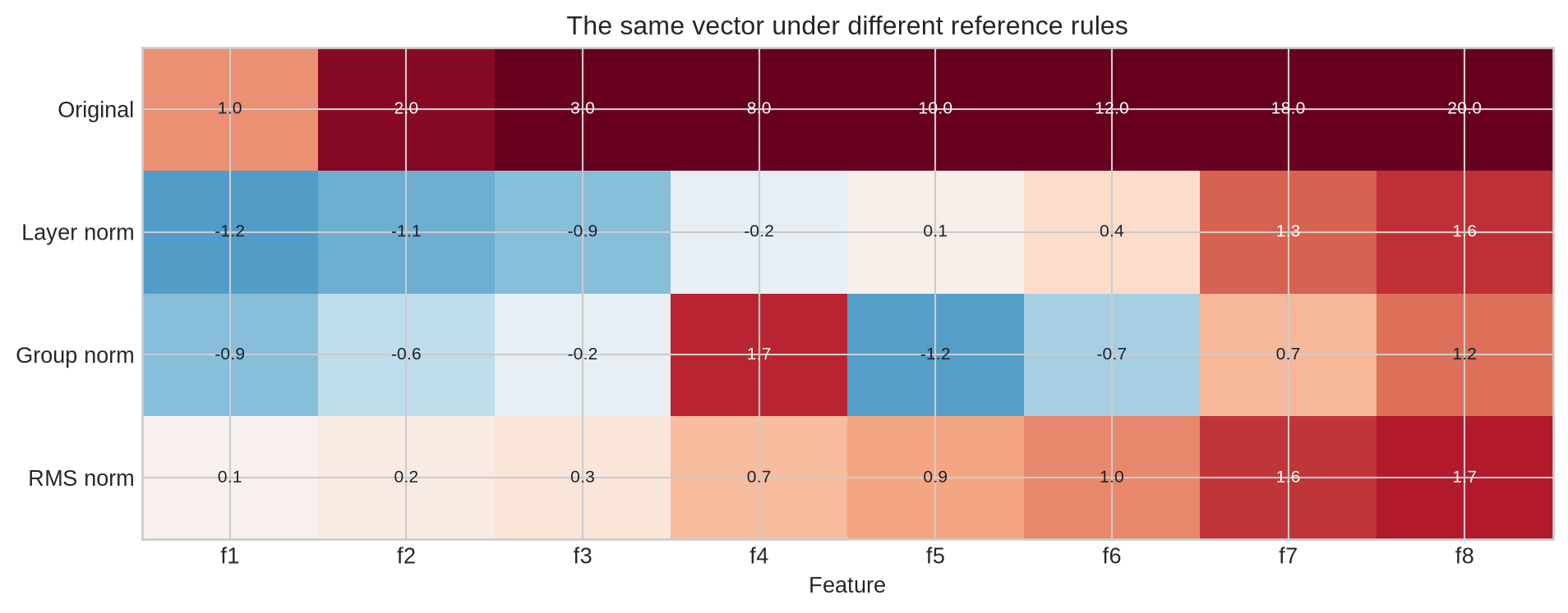
```{python}
#| label: fig-method-comparison
#| fig-cap: "Layer, group, and RMS normalisation retain different information from the same feature vector."
#| fig-alt: "A heatmap compares one original eight-feature vector with layer-normalised, two-group-normalised, and RMS-normalised versions."
sample = np.array([[1., 2., 3., 8., 10., 12., 18., 20.]])
layer = standardise(sample, axis=1)
group = sample.reshape(1, 2, 4)
group = standardise(group, axis=2).reshape(1, 8)
rms = sample / np.sqrt(np.mean(sample**2, axis=1, keepdims=True) + 1e-5)
methods = np.vstack([sample, layer, group, rms])

fig, ax = plt.subplots(figsize=(10, 4))
image = ax.imshow(methods, cmap="RdBu_r", aspect="auto", vmin=-2.2, vmax=2.2)
for i in range(methods.shape[0]):
    for j in range(methods.shape[1]):
        ax.text(j, i, f"{methods[i,j]:.1f}", ha="center", va="center", fontsize=8,
                color="white" if abs(methods[i,j]) > 1.25 else "#18242f")
ax.set_yticks(range(4), ["Original", "Layer norm", "Group norm", "RMS norm"])
ax.set_xticks(range(8), [f"f{j+1}" for j in range(8)])
ax.set_xlabel("Feature"); ax.set_title("The same vector under different reference rules")
plt.tight_layout(); plt.show()
```
Layer normalisation centres all eight features together. Group normalisation centres the first four and final four separately, so it removes differences between group means. RMS normalisation controls magnitude but keeps every positive component positive because it does not recenter the vector.
The operational differences are reduction choices over concrete tensor axes. Level 3 writes those reductions explicitly and uses code to verify the resulting shapes and dependencies.
## Level 3 - Mathematics & Code
### Batch and layer normalisation exchange the reduction index
Let $X\in\mathbb{R}^{B\times D}$ contain $B$ observations and $D$ features. Batch normalisation calculates one mean and variance for each feature $j$:
$$
\mu_j=\frac{1}{B}\sum_{i=1}^{B}X_{ij},\qquad
\sigma_j^2=\frac{1}{B}\sum_{i=1}^{B}(X_{ij}-\mu_j)^2.
$$
It then produces
$$
Y_{ij}=\gamma_j\frac{X_{ij}-\mu_j}{\sqrt{\sigma_j^2+\varepsilon}}+\beta_j.
$$
The index $i$ is reduced: all observations contribute to the statistic for feature $j$. The learned $γ_j$ and $β_j$ are shared across observations.
Layer normalisation instead calculates statistics for each observation $i$:
$$
\mu_i=\frac{1}{D}\sum_{j=1}^{D}X_{ij},\qquad
\sigma_i^2=\frac{1}{D}\sum_{j=1}^{D}(X_{ij}-\mu_i)^2.
$$
Now the feature index $j$ is reduced. For sequence data with shape batch $\times$ tokens $\times$ features, layer normalisation is ordinarily applied across features for each token separately. The token does not borrow statistics from other tokens or other sequences.
```{python}
def batch_norm_manual(x, gamma, beta, eps=1e-5):
    mean = x.mean(axis=0, keepdims=True)
    variance = x.var(axis=0, keepdims=True)
    return gamma * (x - mean) / np.sqrt(variance + eps) + beta

def layer_norm_manual(x, gamma, beta, eps=1e-5):
    mean = x.mean(axis=-1, keepdims=True)
    variance = x.var(axis=-1, keepdims=True)
    return gamma * (x - mean) / np.sqrt(variance + eps) + beta

gamma = np.ones((1, X.shape[1]))
beta = np.zeros((1, X.shape[1]))
print("Batch-norm column means:", batch_norm_manual(X, gamma, beta).mean(axis=0).round(5))
print("Layer-norm row means:", layer_norm_manual(X, gamma, beta).mean(axis=1).round(5))
```
The zeros appear along different axes. Checking only the global mean would miss this distinction and could allow a tensor-layout error to pass unnoticed.
### Group normalisation defines intermediate reduction sets
For an image-like tensor with shape $N\times C\times H\times W$, group normalisation partitions the $C$ channels into $G$ groups. Each sample and group obtains statistics across its $C/G$ channels and all spatial positions. Setting $G=1$ resembles layer-wise normalisation across channels and space; setting $G=C$ gives one channel per group, related to instance normalisation. The exact axes, rather than the method name alone, define the operation.
### RMS normalisation removes recentring
For a feature vector $x_i\in\mathbb{R}^{D}$, define
$$
r_i=\sqrt{\frac{1}{D}\sum_{j=1}^{D}x_{ij}^{2}+\varepsilon},\qquad
y_{ij}=\gamma_j\frac{x_{ij}}{r_i}.
$$
There is no $μ_i$ and commonly no learned beta. RMS normalisation therefore provides re-scaling invariance but not re-centring invariance. The distinction matters when a vector's mean carries information or when reducing arithmetic and memory movement is valuable.
```{python}
def rms_norm_manual(x, weight, eps=1e-5):
    rms = np.sqrt(np.mean(x**2, axis=-1, keepdims=True) + eps)
    return weight * x / rms

shifted = np.array([[2., 3., 4., 5.]])
print("Layer norm:      ", layer_norm_manual(shifted, np.ones((1,4)), np.zeros((1,4))).round(3))
print("RMS norm:        ", rms_norm_manual(shifted, np.ones((1,4))).round(3))
print("RMS output mean: ", rms_norm_manual(shifted, np.ones((1,4))).mean().round(3))
```
Layer normalisation removes the common offset and produces positive and negative deviations. RMS normalisation retains the positive offset while controlling the vector's quadratic magnitude.
### PyTorch encodes axes in the module configuration
```{python}
import torch
from torch import nn

torch.manual_seed(12)
batch = torch.tensor(X, dtype=torch.float32)
bn = nn.BatchNorm1d(4, affine=True)
ln = nn.LayerNorm(4, elementwise_affine=True)

bn.train()
bn_training = bn(batch)
ln_output = ln(batch)
bn.eval()
bn_evaluation = bn(batch)

print("Training BN feature means:", bn_training.mean(dim=0).detach().numpy().round(4))
print("LayerNorm observation means:", ln_output.mean(dim=1).detach().numpy().round(4))
print("BN train/eval outputs equal:", torch.allclose(bn_training, bn_evaluation))
```
The final result is false because the evaluation calculation uses running estimates accumulated by the module, while the training calculation uses the current batch. With real training, running estimates aggregate information over many batches. A freshly created layer has seen only the single batch used here.
```{python}
class ManualRMSNorm(nn.Module):
    def __init__(self, dimension, eps=1e-6):
        super().__init__()
        self.weight = nn.Parameter(torch.ones(dimension))
        self.eps = eps

    def forward(self, x):
        scale = torch.rsqrt(x.pow(2).mean(dim=-1, keepdim=True) + self.eps)
        return x * scale * self.weight

sequence = torch.randn(2, 5, 8)  # batch, tokens, features
output = ManualRMSNorm(8)(sequence)
print("Input shape:", tuple(sequence.shape), "Output shape:", tuple(output.shape))
print("Mean output RMS:", output.pow(2).mean(dim=-1).sqrt().mean().item())
```
The module preserves the tensor shape and normalises each token over its final feature dimension. The mean output RMS is near one because the weight begins at one. Training can change that weight independently for each feature.
### Gradients reveal the dependency structure
Under batch normalisation, the output for observation $i$ depends on the batch mean and variance, which depend on every observation. Its gradient therefore contains cross-observation terms. Under layer or RMS normalisation, gradients couple features within one observation but not separate observations. This is why splitting a batch across devices can change ordinary batch-normalised training unless statistics are synchronized.
Level 3 makes the methods precise through indices and axes. Level 4 asks how those choices behave in research architectures and production systems.
## Level 4 - Research & Systems
### The original motivation is not the only explanation
Batch normalisation was introduced as a method for reducing changes in intermediate activation distributions during training, described as internal covariate shift [@ioffe2015batchnorm]. It also changes optimisation geometry, permits larger learning rates in many settings, and injects noise through mini-batch statistics. It is therefore safer to describe its measured effects in a particular model than to treat one proposed mechanism as a universal explanation.
Batch normalisation became especially influential in convolutional networks, where a channel's statistics can be estimated across batch and spatial dimensions. Its dependence on batch composition is less convenient for recurrent and autoregressive computation, where sequence lengths, ordering, and batch sizes vary.
### Architecture changes the sensible reference set
Layer normalisation was designed to avoid mini-batch dependence and became a standard component of Transformer architectures [@ba2016layernorm; @vaswani2017]. A Transformer typically normalises each token's hidden vector. Whether normalisation appears before or after an attention or feed-forward sublayer changes residual-path gradient flow; Chapter 22 will examine that architectural choice rather than treating it as a detail of this chapter.
Group normalisation was developed for settings in which small per-device image batches make batch estimates unstable [@wu2018groupnorm]. The number of groups is a modelling choice: more groups use smaller reference sets and remove scale information more locally. RMS normalisation omits mean subtraction and reduces the operations required for the core calculation [@zhang2019rmsnorm]. Its use in language models should still be evaluated as part of the full residual architecture, not as an isolated substitution.
### Distributed training makes statistics a systems decision
Data-parallel workers ordinarily hold different mini-batches. Local batch normalisation gives each worker different statistics; synchronized batch normalisation communicates sums and squared sums so that workers share a larger reference set. The latter more closely approximates a global batch but introduces collective communication into the forward pass. Group, layer, and RMS normalisation avoid cross-worker statistics and are easier to combine with changing micro-batch sizes.
Gradient accumulation does not automatically enlarge the batch-normalisation reference set. Several micro-batches may contribute to one optimiser update, but each forward pass still calculates its own statistics unless the implementation explicitly does otherwise. The optimiser's effective batch size and the normalisation layer's statistical batch size are distinct quantities.
### Tensor layout, masking, and precision are part of correctness
A normalisation implementation should state the tensor shape and reduction axes. Confusing channels-first and channels-last layouts can normalise the wrong dimension while preserving the expected output shape. In sequence models, padding tokens must not contaminate a statistic when the method reduces across token positions. Standard per-token layer normalisation does not reduce across tokens, so padding elsewhere in the sequence does not enter its statistic.
Means and variances are reduction operations. Implementations often accumulate them in higher precision than the input tensor, particularly under mixed-precision training. Epsilon must be large enough to stabilise low-variance groups but not so large that it dominates the actual variance. Fused kernels can combine normalisation, affine transformation, and residual operations to reduce memory traffic, but fusion makes numerical comparisons and debugging tolerances important.
### A normalisation audit tests dependencies, not only moments
An audit should record the method, reduction axes, epsilon, affine parameters, training or evaluation mode, running-statistic momentum, tensor layout, batch size per device, synchronization, precision, and treatment of padding. It should report realised means, variances or RMS values along the intended axes and inspect gamma and beta during training.
Two perturbation tests are especially informative. First, alter another observation in the batch and check whether the target observation changes; this exposes unintended cross-observation dependence. Second, run the same target alone, in a different batch, and in evaluation mode. The resulting differences show whether the deployed function matches the assumed reference rule.
Normalisation does not guarantee stable optimisation. It interacts with initialisation, residual scaling, optimiser settings, activation functions, and data distribution. The relevant evidence is the behaviour of the complete implemented path.
## Common misconceptions
- **Normalisation means dividing all model inputs by one global standard deviation.** Different methods choose different reference sets and can operate on intermediate activations.
- **Every normalised output has global mean zero and variance one.** The property holds along selected axes before the learned affine transformation.
- **Gamma and beta undo normalisation completely.** They restore feature-wise scale and shift, but not the individual means and variances removed from each reference set.
- **Batch normalisation uses the current batch at inference.** Standard evaluation uses stored running statistics.
- **Gradient accumulation gives batch normalisation a larger statistical batch.** Each forward micro-batch ordinarily has its own statistics.
- **Layer normalisation normalises across tokens.** In Transformers it normally reduces across the hidden features of each token.
- **RMS normalisation is layer normalisation with a different epsilon.** It omits mean subtraction and usually the additive bias.
- **Group normalisation is independent of axis choices.** Its meaning depends on channel grouping and tensor layout.
- **Normalisation removes the need for careful initialisation.** It changes signal propagation but does not remove architecture-wide stability requirements.
- **A numerically finite output proves the layer is configured correctly.** The wrong reduction axis can produce finite, plausible values.
- **Training and evaluation modes differ only for dropout.** Batch normalisation also changes its source of statistics.
- **Synchronized batch normalisation is free.** It introduces communication into every normalised forward pass.
## Exercises
1. For the first column of the running matrix, calculate the batch mean, variance, and normalised value of $X_{31}=4$.
2. Calculate the layer-normalised values for the first row.
3. Explain why changing the final row affects the batch-normalised first row but not its layer-normalised result.
4. Apply $γ=2$ and $β=-1$ to a standardised value of $0.5$ and interpret the result.
5. Show what epsilon prevents when all values in a reference set are identical.
6. Reproduce the batch-size simulation for variance estimates rather than means.
7. Compare batch-normalised outputs for one target observation placed in three different mini-batches.
8. Explain why evaluation mode should produce a stable prediction for a fixed observation.
9. Write reduction axes for batch normalisation on an $N\times C\times H\times W$ image tensor.
10. Calculate two-group normalisation for an eight-channel vector.
11. Compare layer and RMS normalisation after adding the same constant to every feature.
12. Implement a masked normalisation across sequence positions and test it with padding.
13. Inspect PyTorch running means across 20 deliberately shifted mini-batches.
14. Test whether gradient accumulation changes per-micro-batch statistics.
15. Design an audit for normalisation in a mixed-precision, data-parallel model.
16. A Transformer implementation replaces layer normalisation with RMS normalisation. State one statistic that is no longer centred, one statistic that is still controlled, and one fixed-input test that would reveal the implemented reduction axes.
## Summary
Normalisation expresses activations relative to a selected reference set. Batch normalisation reduces across observations for each feature and therefore introduces batch dependence. Layer normalisation reduces across features within one observation or token. Group normalisation uses intermediate channel groups. RMS normalisation controls root-mean-square magnitude without subtracting a mean.
The shared computational pattern is simple: calculate statistics, transform the activations, and apply learned scale or shift. The implications are not simple. Reduction axes determine which values influence one another; batch normalisation requires separate training and evaluation behaviour; small batches create noisy statistics; and distributed execution can require communication. Tensor layout, padding, epsilon, and accumulation precision are part of the method's correctness.
The appropriate method follows from the dependency the architecture can support. A name in a configuration file is insufficient evidence. Realised axis-wise statistics and perturbation tests show what the implementation actually does.
## Looking ahead
Chapter 13 examines optimisers and learning-rate schedules. Normalisation changes the scale and geometry encountered by the optimiser; the next chapter studies how gradients are converted into parameter updates over time.
## Further reading
Batch normalisation was introduced by @ioffe2015batchnorm. Observation-wise layer normalisation is developed by @ba2016layernorm. @wu2018groupnorm analyse group normalisation under small image batches. RMS normalisation is introduced by @zhang2019rmsnorm. The original Transformer provides an important architectural application of layer normalisation [@vaswani2017].