---
title: "Mixture-of-experts Models"
subtitle: "Sparse routing, expert capacity, load balancing, and systems cost"
---
## Chapter orientation
### Why this chapter matters
A dense Transformer applies the same feed-forward parameters to every token. Increasing its capacity therefore increases the computation and memory required for every token. A mixture-of-experts (MoE) layer replaces one feed-forward subnetwork with several experts and a router that activates only a small subset for each token. The model can contain many more parameters than a comparably priced dense layer, while its active computation remains bounded by the selected experts.
That arithmetic is incomplete. A useful MoE layer must decide which experts receive which tokens, prevent a few experts from receiving most of the work, and move token representations to the devices that hold the selected experts. Routing and communication are therefore part of the model, not implementation detail. This chapter establishes those mechanisms before the later chapters on serving, monitoring, and safety.
### Learning objectives
By the end of this chapter, you should be able to:
- distinguish total parameters from active parameters per token;
- describe router scores, top- k selection, expert outputs, and weighted combination;
- calculate a toy expert-capacity limit and identify dropped or rerouted tokens;
- explain why load balancing changes both training and systems behaviour;
- compare dense and MoE cost under a stated routing policy; and
- specify an MoE evaluation and deployment record.
### Running layer
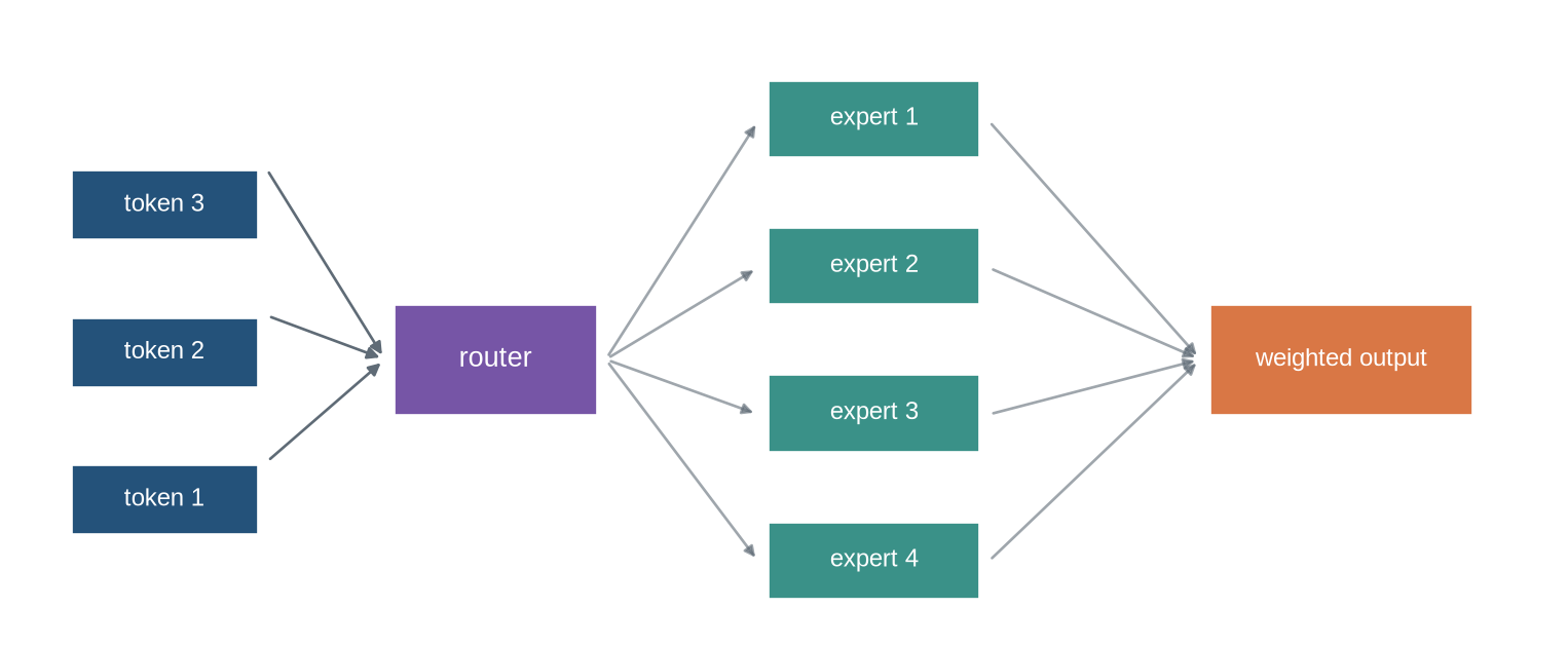
The running example has four feed-forward experts and a router that selects two per token. The numbers are deliberately small so that routing, capacity, and aggregation can be inspected directly.
```{python}
#| label: fig-moe-layer
#| fig-cap: "An MoE layer routes each token to a small subset of experts, combines their outputs, and leaves the remaining experts inactive for that token."
#| fig-alt: "Three token representations enter a router; each is sent to two of four expert boxes before weighted outputs are combined."
import numpy as np
import matplotlib.pyplot as plt
from matplotlib.patches import Rectangle, FancyArrowPatch
plt.style.use("seaborn-v0_8-whitegrid")
blue,teal,orange,purple,grey="#24527a","#3a9188","#d97745","#7655a6","#5f6b76"
fig,ax=plt.subplots(figsize=(10,4)); ax.axis("off")
for i in range(3):
    ax.add_patch(Rectangle((.3,.7+i*.8),1.1,.38,facecolor=blue,edgecolor="white")); ax.text(.85,.89+i*.8,f"token {i+1}",ha="center",va="center",color="white",fontsize=9)
ax.add_patch(Rectangle((2.2,1.35),1.2,.6,facecolor=purple,edgecolor="white")); ax.text(2.8,1.65,"router",ha="center",va="center",color="white")
for i in range(4):
    ax.add_patch(Rectangle((4.4,2.75-i*.8),1.25,.42,facecolor=teal,edgecolor="white")); ax.text(5.03,2.96-i*.8,f"expert {i+1}",ha="center",va="center",color="white",fontsize=9)
ax.add_patch(Rectangle((7.0,1.35),1.55,.6,facecolor=orange,edgecolor="white")); ax.text(7.78,1.65,"weighted output",ha="center",va="center",color="white",fontsize=9)
for y in [1.09,1.89,2.69]: ax.add_patch(FancyArrowPatch((1.45,y),(2.15,1.65),arrowstyle="-|>",color=grey,mutation_scale=9))
for y in [2.95,2.15,1.35,.55]: ax.add_patch(FancyArrowPatch((3.45,1.65),(4.35,y),arrowstyle="-|>",color=grey,mutation_scale=8,alpha=.6))
for y in [2.95,2.15,1.35,.55]: ax.add_patch(FancyArrowPatch((5.7,y),(6.95,1.65),arrowstyle="-|>",color=grey,mutation_scale=8,alpha=.6))
ax.set_xlim(0,9); ax.set_ylim(.2,3.5); plt.show()
```
::: {.concept-box .concept-core #concept-moe data-term="Mixture of experts" data-domain="Modern AI systems"}
**Mixture of experts.** A model with specialised expert modules selected by a router for each input or token. Total parameters, active parameters, capacity, routing load, and communication together determine its behaviour and cost.
:::
## Level 1 - Intuition
### Capacity can grow without activating every parameter
The dense layer asks one feed-forward network to process every token. An MoE layer gives the router several such networks and lets it select specialists conditionally. A token associated with code-like text may be routed differently from a token in another language or a mathematical expression. The system does not need a semantic story about each expert for this to be useful; the operational claim is that different tokens activate different parameter subsets.
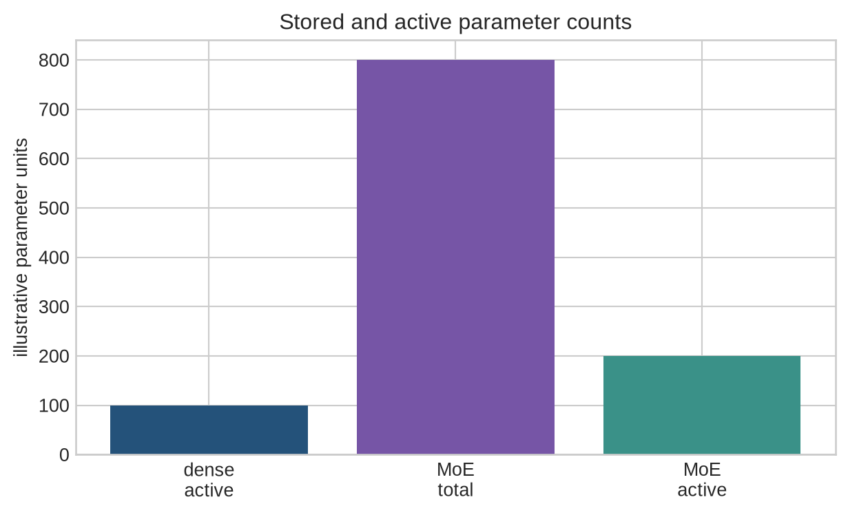
Sparse activation changes the comparison. A model with eight experts may store roughly eight feed-forward parameter sets, but a top-2 router only executes two for one token. Parameter count therefore measures stored capacity, while active parameters and communication determine per-token cost. The sparsely gated MoE layer formalised this conditional-computation approach, and subsequent work made routing simple enough to support large Transformer training [@shazeer2017moe; @fedus2021switch].
```{python}
dense_parameters=100
experts,active=8,2
print({"dense_active":dense_parameters,"moe_total":experts*dense_parameters,"moe_active":active*dense_parameters})
```
```{python}
#| label: fig-total-active-parameters
#| fig-cap: "An MoE layer can increase stored parameter capacity while keeping the active expert count per token fixed."
#| fig-alt: "Bars compare dense active parameters with total and active parameters for an eight-expert top-two MoE layer."
labels=["dense\nactive","MoE\ntotal","MoE\nactive"]; values=[100,800,200]
fig,ax=plt.subplots(figsize=(6.5,4)); ax.bar(labels,values,color=[blue,purple,teal]); ax.set_ylabel("illustrative parameter units")
ax.set_title("Stored and active parameter counts"); plt.tight_layout(); plt.show()
```
### Routing is conditional on a token and its batch context
The router score is computed from a token representation, but the realised dispatch can depend on the surrounding batch. Capacity limits, token order, expert-parallel layout, and tie handling determine which selected assignments are actually processed when several tokens request the same expert. Two copies of the same token can therefore receive different fallback treatment in different batches even when their router scores are unchanged. A routing claim should distinguish the score produced by the router from the assignment that reached an expert.
This distinction matters for reproducibility. Record the batching and packing policy, sequence lengths, top-k rule, capacity factor, token ordering where relevant, and whether assignment is deterministic under a fixed seed. An average routing histogram can conceal a capacity conflict that occurs only in long sequences or one language slice. The relevant unit for systems evaluation is the realised assignment and its outcome, not only the router's preferred expert.
## Level 2 - Routing and capacity mechanics
### Router scores become a sparse dispatch decision
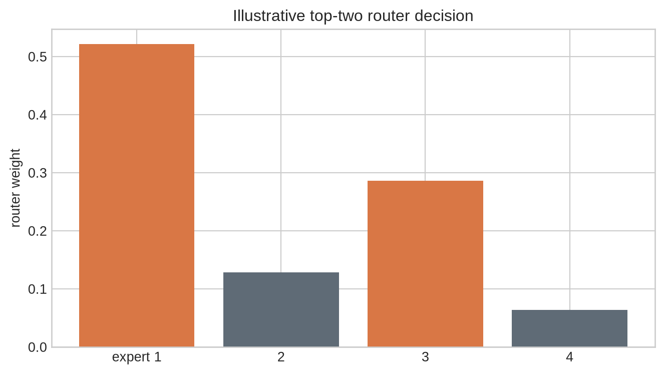
For token representation (x), a router produces one score per expert. A softmax can turn the scores into non-negative weights. Top- k routing retains only the k largest weights, renormalises them, sends the token to those experts, and combines their outputs. If experts are functions (f_e), the layer output is the weighted sum of the selected (f_e(x)). This is conditional computation: routing determines which parameters participate in this token's forward and backward pass.
```{python}
scores=np.array([1.8,.4,1.2,-.3])
weights=np.exp(scores-scores.max()); weights=weights/weights.sum()
chosen=np.argsort(weights)[-2:]; selected=weights[chosen]/weights[chosen].sum()
print("router weights:",np.round(weights,3),"experts:",chosen,"renormalised:",np.round(selected,3))
```
```{python}
#| label: fig-topk-routing
#| fig-cap: "Top-k routing retains the largest router weights and renormalises only the selected experts before their outputs are combined."
#| fig-alt: "A bar chart shows four router weights, highlighting the two selected experts and their renormalised weights."
fig,ax=plt.subplots(figsize=(7,4)); colours=[orange if i in chosen else grey for i in range(4)]
ax.bar(range(4),weights,color=colours); ax.set_xticks(range(4),["expert 1","2","3","4"]); ax.set_ylabel("router weight")
ax.set_title("Illustrative top-two router decision"); plt.tight_layout(); plt.show()
```
### Top-k selection has ties, normalisation, and gradient consequences
Top-k creates a discontinuous membership decision: an expert just below the cutoff receives no expert computation for that token, while one just above it receives a renormalised weight. Ties and near-ties therefore require a deterministic or recorded tie rule. The selected weights should sum to one if the implementation defines a weighted combination, but the unselected router scores can still matter for the router's learning signal and auxiliary objectives.
The router and experts also receive different gradients. Selected experts receive token-specific gradients; unselected experts do not receive that token's expert-path gradient. Router updates depend on the routing formulation and losses used to encourage balance or exploration. These are reasons to report router settings separately from the feed-forward expert architecture. A change in top-k or normalisation affects both the active computation and the data each expert sees during training.
Report these choices with the checkpoint, training batch policy, and evaluator version.
### Capacity limits make dispatch observable
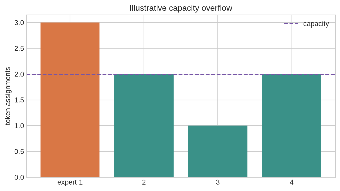
Experts cannot process an unlimited number of token assignments in one batch. A capacity factor sets a per-expert quota relative to the average expected load. When an expert is full, the implementation may drop an assignment, send it to a backup expert, or preserve a residual path. Each choice changes the layer output and must be reported. A low capacity limit raises the chance of discarded routes; a high limit reserves memory and can leave accelerator work uneven.
```{python}
assignments=np.array([0,0,0,1,1,2,3,3]); capacity=2
counts=np.bincount(assignments,minlength=4); overflow=np.maximum(counts-capacity,0)
print("expert loads:",counts,"overflow:",overflow)
```
```{python}
#| label: fig-expert-capacity
#| fig-cap: "Expert capacity limits turn unequal router demand into overflow that must be dropped, rerouted, or handled by a declared fallback."
#| fig-alt: "Four bars show expert token loads against a horizontal capacity limit; the first expert exceeds the line."
fig,ax=plt.subplots(figsize=(7,4)); ax.bar(range(4),counts,color=[orange if c>capacity else teal for c in counts])
ax.axhline(capacity,color=purple,linestyle="--",label="capacity"); ax.set_xticks(range(4),["expert 1","2","3","4"]); ax.set_ylabel("token assignments"); ax.legend()
ax.set_title("Illustrative capacity overflow"); plt.tight_layout(); plt.show()
```
### Overflow handling defines an output contract
Dropping an assignment, rerouting it to a lower-ranked expert, or using a residual dense path are different model behaviours. Dropping can reduce computation but may remove information from a token's update. Rerouting can retain an expert computation while changing the router's intended choice. A residual path can preserve a dense fallback but changes the active-parameter and cost comparison. There is no neutral overflow policy.
The overflow record should therefore include the selected experts, successful assignments, fallback type, and the final path used for each affected token. Measure overflow separately from router entropy or load balance: a router can look balanced on average while still producing concentrated conflicts at the capacity boundary. Evaluate overflow on held-out batches and changed sequence-length distributions, because a capacity factor chosen on one workload may fail on another.
## Level 3 - Training and systems constraints
### Load balancing supplies a training signal and a hardware constraint
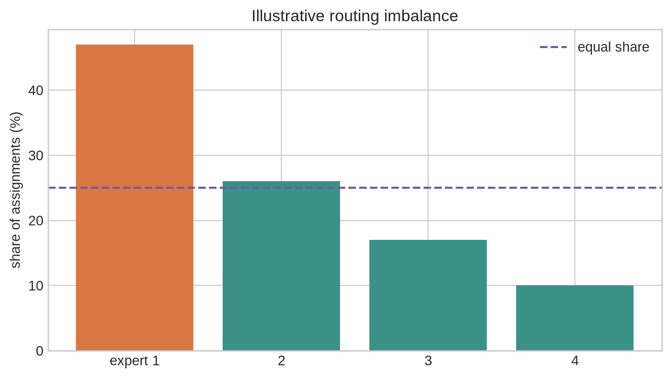
If a router repeatedly selects one expert, that expert becomes a bottleneck while other experts receive little data or gradient signal. MoE training commonly adds an auxiliary load-balancing objective based on routing probabilities and realised assignments. The objective encourages use of the available experts; it does not prove that expert specialisation is meaningful or that all experts should receive identical traffic.
The systems consequence is immediate. Tokens assigned to experts on other devices must be exchanged, processed, and returned. The slowest or most overloaded expert can determine the layer's step time. GShard treated conditional computation and sharding together because large MoE training requires both a routing rule and an execution plan [@lepikhin2020gshard].
```{python}
loads=np.array([47,26,17,10]); uniform=np.repeat(25,4)
print("absolute deviation from equal load:",np.abs(loads-uniform).sum())
```
```{python}
#| label: fig-load-balance
#| fig-cap: "Unequal expert load leaves some experts underused and makes the busiest expert a capacity and latency bottleneck."
#| fig-alt: "A bar chart compares uneven token shares across four experts with a horizontal equal-share line."
fig,ax=plt.subplots(figsize=(7,4)); ax.bar(range(4),loads,color=[orange,teal,teal,teal]); ax.axhline(25,color=purple,linestyle="--",label="equal share")
ax.set_xticks(range(4),["expert 1","2","3","4"]); ax.set_ylabel("share of assignments (%)"); ax.legend(); ax.set_title("Illustrative routing imbalance")
plt.tight_layout(); plt.show()
```
### Load balancing has probability, assignment, and quality diagnostics
The router's average probability mass and the realised token assignments are related but not identical. A load-balancing loss can encourage probability mass to spread across experts while top-k selection and capacity constraints still produce uneven realised loads. Report both quantities, together with overflow, expert utilisation, duplicate selections, and the coefficient of variation or another stated imbalance measure. A single auxiliary-loss value is not evidence that the dispatch is balanced.
Balance also has a quality boundary. Equal traffic can be undesirable if a subset of tasks genuinely needs a particular expert and the balance penalty forces it elsewhere. Conversely, concentrated traffic may expose an expert to a narrow data slice and leave other experts poorly trained. Compare task outcome and routing diagnostics as the balance coefficient changes, keeping the rest of the training contract fixed. Sparse-routing systems such as GShard and Switch Transformers make these routing and capacity choices part of the training design, not a post-training serving adjustment [@lepikhin2020gshard; @fedus2021switch].
### A dense comparison requires an end-to-end cost record
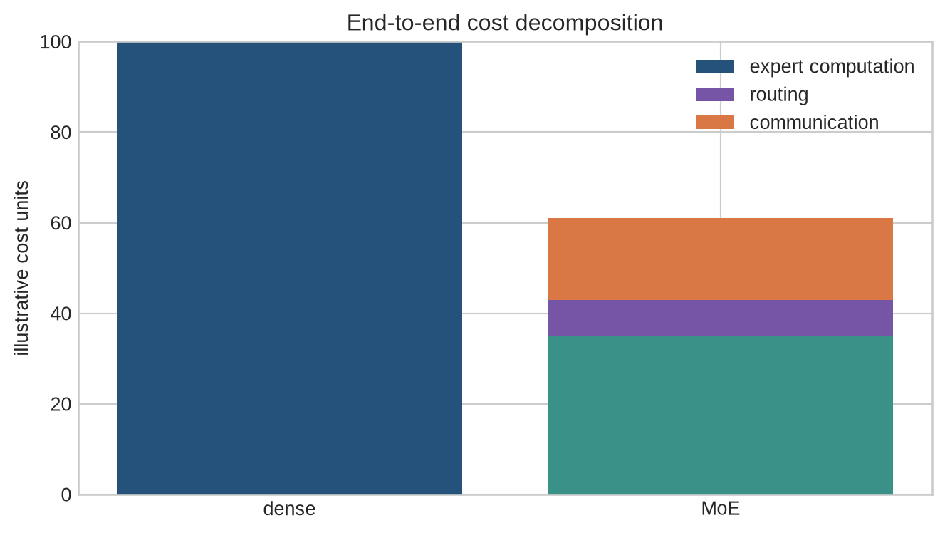
MoE can reduce active feed-forward computation for a given stored capacity, but it can also add router work, dispatch overhead, all-to-all communication, padding to expert capacity, and latency variation across requests. Compare dense and sparse models under the same sequence lengths, batch policy, precision, hardware, and quality metric. A parameter count alone cannot establish a serving advantage.
```{python}
systems={"dense":{"compute":100,"communication":0,"latency":12},"moe":{"compute":35,"communication":18,"latency":14}}
for name,record in systems.items(): print(name,record)
```
### Dispatch has a topology and a synchronisation cost
In an expert-parallel layout, a token may need to leave the device that computed its shared attention representation, be grouped with tokens for its selected expert, and return before the next shared layer. The cost depends on the device placement of experts, communication links, token imbalance, message sizes, and the slowest participating device. All-to-all exchange can make the latency of a layer depend on a small overloaded expert even when the average active computation is low.
Measure dispatch separately from expert matrix multiplication. A useful systems record includes expert-to-device placement, number of devices, communication volume, padding induced by capacity, collective-operation timing, and tail rather than only mean latency. Distributed training and model-parallel work supplies the relevant distinction between local computation and communication or synchronisation cost [@li2020ddp; @narayanan2021megatron]. The same distinction applies when comparing a sparse layer with a dense layer on a declared hardware topology.
```{python}
#| label: fig-cost-decomposition
#| fig-cap: "MoE active expert computation can be lower than a dense comparison while routing and communication add to the end-to-end latency budget."
#| fig-alt: "Stacked bars compare illustrative dense compute with MoE expert compute, routing, and communication costs."
fig,ax=plt.subplots(figsize=(7,4)); ax.bar(["dense","MoE"],[100,35],color=[blue,teal],label="expert computation")
ax.bar(["dense","MoE"],[0,8],bottom=[100,35],color=purple,label="routing")
ax.bar(["dense","MoE"],[0,18],bottom=[100,43],color=orange,label="communication")
ax.set_ylabel("illustrative cost units"); ax.legend(); ax.set_title("End-to-end cost decomposition"); plt.tight_layout(); plt.show()
```
## Level 4 - Evaluation, deployment, and limits
### Evaluate routing as well as task output
An MoE report should include task quality, total and active parameters, experts and top-k, routing distribution, capacity factor, overflow or fallback rate, auxiliary-loss weight, sequence length, batch size, precision, hardware topology, communication volume, throughput, and latency distribution. Report these by input slice where routing differs across languages, lengths, or domains. Aggregate accuracy can conceal an expert that is overloaded only for a small but important set of inputs.
Expert labels should also be interpreted cautiously. Similar token clusters in one expert can be a useful diagnostic; they do not establish a stable semantic role, causal explanation, or fairness property. Rerouting, changing capacity, or changing the batch can alter the traffic observed by an expert. The appropriate claim concerns the measured routing policy and workload.
### Evaluate routing changes with matched quality and workload slices
An MoE intervention can change top-k, capacity factor, balance coefficient, overflow fallback, expert count, or device placement. Evaluate one such change at a time under the same checkpoint where possible, input distribution, sequence lengths, batch policy, precision, and quality scorer. Report task outcome together with overflow, routed fraction, per-expert load, communication, p50 and p95 latency, and memory. A throughput gain that relies on dropping more assignments or a quality gain that relies on a larger batch is not a routing result alone.
Slice the record by properties that plausibly change routing: language, input length, token class, domain, tool-call format, or a declared sensitive workload category. The purpose is not to assign an expert a human-readable identity. It is to discover whether the routing policy creates concentrated overflow, latency, or quality loss for a subset that aggregate results hide. A deployment decision can then adjust capacity, routing, or fallback for the affected workload rather than treating a global average as sufficient evidence.
```{python}
record={"experts":8,"top_k":2,"capacity_factor":1.25,"overflow_rate":.03,"load_cv":.31,"p95_latency_ms":28,"quality":"held-out exact match"}
assert {"experts","top_k","overflow_rate","p95_latency_ms","quality"} <= set(record)
print("MoE evaluation record complete")
```
## Common misconceptions
- **An MoE uses all of its parameters for every token.** Routing activates only the selected experts.
- **More total parameters imply proportionally more per-token computation.** Active experts, routing, and communication determine the relevant cost.
- **Load balancing makes experts interchangeable.** It changes traffic incentives; it does not establish what each expert represents.
- **A router is a minor pre-processing step.** It determines computation, gradients, overflow, and communication.
- **Sparse activation guarantees lower serving latency.** Dispatch and cross-device communication can dominate the gain.
## Exercises
1. Distinguish total, active, and shared parameters in a top-two MoE layer.
2. Compute top-two routing weights from four supplied router scores.
3. Explain why selected weights are renormalised.
4. Calculate expert loads and overflow for a toy dispatch table.
5. Compare dropping, rerouting, and residual fallback for an overflow token.
6. State one purpose and one limit of an auxiliary load-balancing objective.
7. Identify a batch property that can change observed expert traffic.
8. Design a routing slice analysis for inputs in two languages.
9. Compare dense and MoE systems under a matched latency record.
10. Explain why active FLOPs do not capture all MoE serving cost.
11. Specify fields required for an MoE evaluation record.
12. Construct a case where equal average expert load hides a tail-latency problem.
13. Explain how a capacity factor changes memory and overflow risk.
14. State why expert specialisation needs evidence beyond a token sample.
15. Design a held-out test for a routing-policy change.
16. Identify which later chapter should own serving and monitoring decisions.
## Summary
Mixture-of-experts layers increase stored capacity through conditional expert activation. Their behaviour depends on router selection, capacity limits, load balance, dispatch, and hardware communication. Evaluate task quality together with the full routing and systems record; sparse parameters alone do not establish an efficiency claim.
## Looking ahead
Sparse routing changes where computation occurs, but it does not change the token interface that the Transformer processes. [Chapter 44](44-vision-transformers.qmd) examines what happens when that interface is built from image patches rather than text tokens, including the positional and data requirements that follow.
## Further reading
The sparsely gated MoE layer is introduced by @shazeer2017moe. GShard studies conditional computation with automatic sharding [@lepikhin2020gshard], and Switch Transformers simplify sparse expert routing for large Transformer training [@fedus2021switch].