Context Windows and Model Inference

Finite prefixes, cached states, and the limits of long-context generation

The problem

Chapter 26 produced a base-model checkpoint fitted to a constructed token stream under a finite training budget. Serving that checkpoint confronts a different constraint. A decoder language model predicts the next token from a finite permitted prefix, and the maximum number of tokens it can process in one request is the context window. That limit affects what evidence is available to a prediction, the memory required by attention, the latency of generation, and the interpretation of claims that a model has “read” a long document.

Inference is also sequential: a generated token becomes part of the next prefix. Key-value caching avoids recomputing the representations of earlier tokens at every step, but it retains an expanding memory state. This chapter defines those mechanics and the evidence needed to assess long-context use. Chapter 28 treats how tokens are selected from the next-token distribution.

A sliding window makes the boundary visible

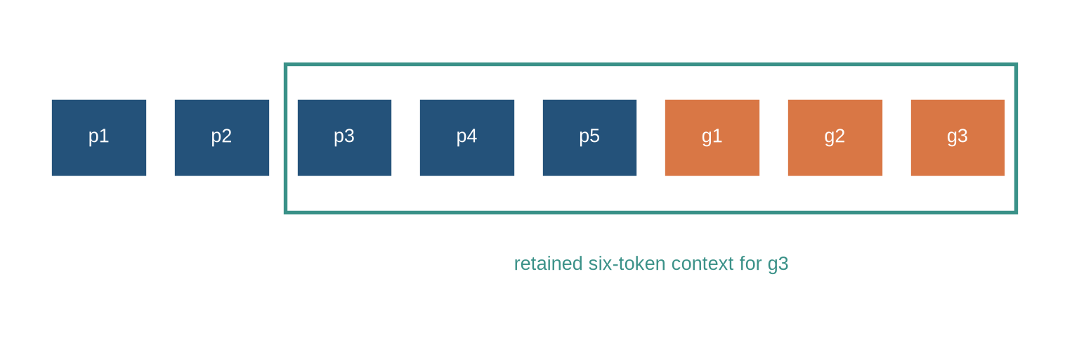
The running sequence uses a prompt of five token IDs and generates three new IDs. A maximum context of six means that a later prediction cannot retain every original prompt token if the system uses a sliding window.

The first diagram shows the whole sequence and the retained window. The blue boxes are prompt tokens and the orange boxes are generated tokens; the outlined span is the six-token context available when the model predicts the final token. Notice that p1 and p2 have left the window: they influenced earlier predictions, but they are no longer available to this one.

import numpy as np
import matplotlib.pyplot as plt
from matplotlib.patches import Rectangle, FancyArrowPatch
plt.style.use("seaborn-v0_8-whitegrid")
blue,teal,orange,purple,grey="#24527a","#3a9188","#d97745","#7655a6","#5f6b76"
tokens=["p1","p2","p3","p4","p5","g1","g2","g3"]
fig,ax=plt.subplots(figsize=(10,3)); ax.axis("off")
for i,t in enumerate(tokens):
    x=.35+i*1.15; c=blue if i<5 else orange
    ax.add_patch(Rectangle((x,1.25),.9,.5,facecolor=c,edgecolor="white")); ax.text(x+.45,1.5,t,ha="center",va="center",color="white")
ax.add_patch(Rectangle((2.55,1.02),6.85,.95,fill=False,edgecolor=teal,lw=2)); ax.text(5.98,.65,"retained six-token context for g3",ha="center",color=teal)
ax.set_xlim(0,9.8); ax.set_ylim(.3,2.3); plt.show()

Figure 28.1: A finite causal context makes each prediction depend on the retained prefix, not necessarily the complete earlier document.

The window is a token limit, not a summary of what the model used: everything inside it is available in principle, and everything outside it is gone. The rest of the chapter separates that capacity from the cost of filling it and from the evidence that a model actually uses what fits.

Context window and key-value cache. The context window is the finite token prefix a model can condition on in one request. A key-value cache stores prior attention states during decoding to avoid recomputation, while consuming memory that grows with active context.

Configured context limit and supported length. A configured limit is the maximum length an implementation accepts. Supported length is the range over which task performance has been evaluated. The first is a setting; the second is an evidence claim.

Level 1 - Intuition

A context window is an information boundary

The context window is a token limit, not a guarantee that every retained token affects an answer. A token outside the window cannot be attended to by an ordinary finite-context decoder. A token inside it is available in principle, but the model may assign it little attention, fail to retrieve it among distractors, or use it incorrectly. “Supports 32,000 tokens” therefore describes an input capacity, not a measured ability to answer questions about every position in a 32,000-token document.

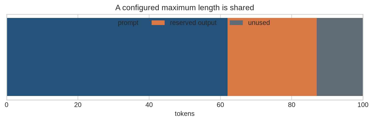
The boundary is measured after tokenisation. A page, a word count, or a character count has no fixed conversion because language, formatting, code, and tokenizer affect the number of IDs. Prompts also consume the same budget as generated output in most interfaces. A requested answer can fail because the prompt plus reserved output exceeds the configured total length.

limit=100; prompt=62; reserve=25
fig,ax=plt.subplots(figsize=(8,2.7)); ax.barh([0],[prompt],color=blue,label="prompt"); ax.barh([0],[reserve],left=[prompt],color=orange,label="reserved output"); ax.barh([0],[limit-prompt-reserve],left=[prompt+reserve],color=grey,label="unused"); ax.set_xlim(0,limit); ax.set_yticks([]); ax.set_xlabel("tokens"); ax.legend(ncol=3,loc="upper center"); ax.set_title("A configured maximum length is shared"); plt.tight_layout(); plt.show()

Figure 28.2: Prompt tokens and generated tokens share a finite total sequence budget.

Prompt processing and generation are different phases

During prompt processing, a causal Transformer can compute representations for supplied positions in parallel under its causal mask. This is commonly called prefill. Once generation begins, token \(t+1\) cannot be selected until the model has processed the selected token \(t\). Output is therefore sequential even on highly parallel hardware.

The difference helps interpret latency. A long prompt can create a substantial initial wait before the first new token. A long generated answer can be slow because it requires repeated decode steps. Reporting only total tokens per second mixes these phases and obscures the user-facing bottleneck.

prompt=np.array([2,11,34,58,3]); generated=[]
for chosen in [17,29,3]:
    print("prefix length before selection:",len(prompt)+len(generated),"choose:",chosen)
    generated.append(chosen)

prefix length before selection: 5 choose: 17
prefix length before selection: 6 choose: 29
prefix length before selection: 7 choose: 3

Level 1 identified the window as an information boundary and the two phases of a request. Level 2 follows the cache that makes sequential generation affordable: why naive decoding repeats work, what the cache stores, and how its correctness is tested.

Level 2 - Mechanics

Why naive decoding repeats work

Without a cache, generating each new token recomputes attention projections for the full prefix. For a prefix length \(L\), the next step uses length \(L+1\), then \(L+2\), and so on. Earlier tokens are repeatedly projected even though their keys and values do not change in a causal decoder.

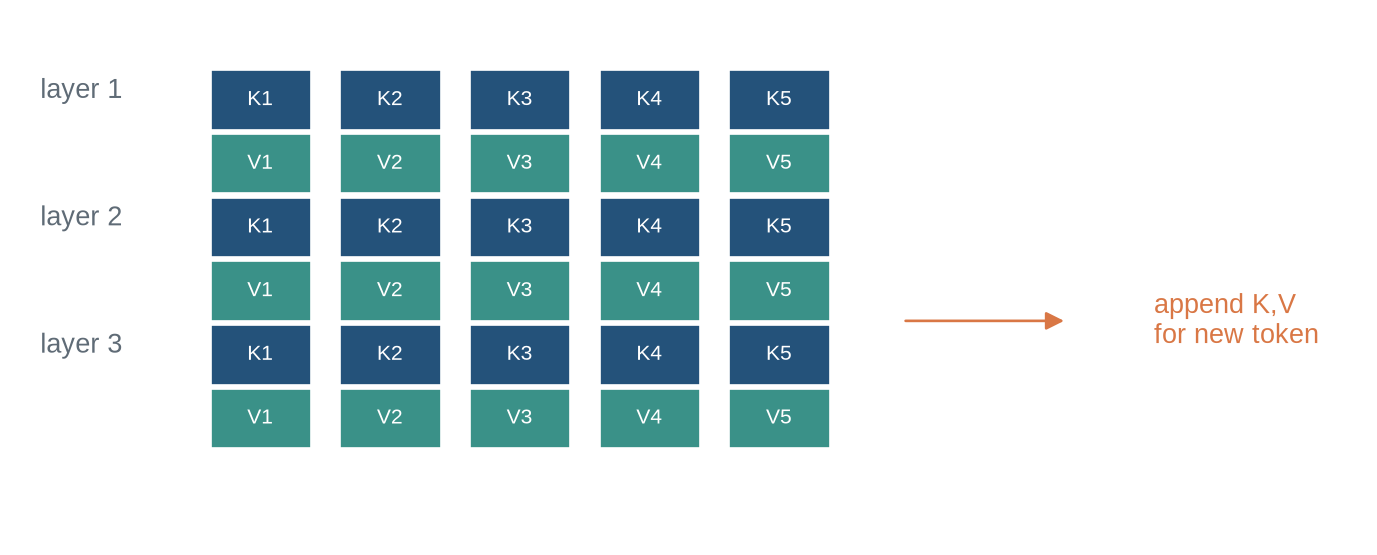
A key-value cache stores the key and value tensors produced at each layer for earlier positions. At the next step, the new query attends to stored keys and values plus the new token’s key and value. The cache does not make generation parallel, but it avoids repeatedly rebuilding the earlier prefix.

fig,ax=plt.subplots(figsize=(9,3.5)); ax.axis("off")
for layer in range(3):
    y=2.65-layer*.8; ax.text(.15,y+.2,f"layer {layer+1}",color=grey)
    for i in range(5):
        x=1.35+i*.92; ax.add_patch(Rectangle((x,y),.72,.38,facecolor=blue,edgecolor="white")); ax.text(x+.36,y+.19,f"K{i+1}",ha="center",va="center",color="white",fontsize=8)
        ax.add_patch(Rectangle((x,y-.4),.72,.38,facecolor=teal,edgecolor="white")); ax.text(x+.36,y-.21,f"V{i+1}",ha="center",va="center",color="white",fontsize=8)
ax.add_patch(FancyArrowPatch((6.25,1.45),(7.45,1.45),arrowstyle="-|>",color=orange,mutation_scale=14)); ax.text(8.05,1.45,"append K,V\nfor new token",va="center",color=orange)
ax.set_xlim(0,9.5); ax.set_ylim(.1,3.35); plt.show()

Figure 28.3: A key-value cache retains keys and values for each layer and each generated prefix position, growing with sequence length.

Cache shape and memory

For batch size \(B\), layers \(n_l\), key-value heads \(n_{kv}\), head width \(d_h\), and cached length \(L\), keys and values require approximately

\[ 2B n_l n_{kv} L d_h \]

stored numbers. Multiply by bytes per number to obtain a rough memory estimate. Multi-query and grouped-query attention reduce \(n_{kv}\) relative to the number of query heads, lowering cache memory without changing the causal sequence rule.

B,layers,kv_heads,length,head_dim,bytes_per=1,32,8,8192,128,2
cache_bytes=2*B*layers*kv_heads*length*head_dim*bytes_per
print(f"KV cache: {cache_bytes/2**30:.2f} GiB")

KV cache: 1.00 GiB

The estimate excludes model weights, activations required by the serving system, allocator overhead, metadata, and temporary attention buffers. It is useful for identifying linear growth with context length, not for replacing a measured memory profile.

Cache correctness is a model test

Cached decoding should agree with full-prefix decoding for the same model, tokens, position treatment, masks, and numerical precision within an explicit tolerance. Disagreement can arise from wrong cache positions, stale entries, incorrect padding handling, rotary-position implementation, or an inconsistency between prefill and decode code paths.

full_prefix_logits=np.array([.1,.2,.7])
cached_logits=np.array([.1,.2,.7])
assert np.allclose(full_prefix_logits,cached_logits,atol=1e-6)
print("cached and full-prefix reference outputs agree")

cached and full-prefix reference outputs agree

Level 2 specified what the cache stores and how its correctness is tested. Level 3 states the cost relations formally: what prefill costs before any cache exists, and how retrieval differs from a longer window.

Level 3 - Mathematics & Code

Cost grows before the cache is available

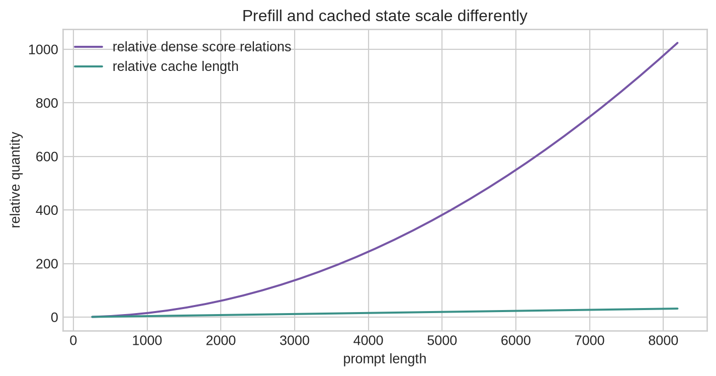
The cache improves repeated decoding but does not remove the cost of processing a long initial prompt. Standard dense self-attention forms score relations among positions during prefill, so the attention component grows quadratically with sequence length. Chapter 20 derived this relation. Implementation methods can reduce memory traffic and avoid materialising the full score matrix, but they do not make every long prompt free.

lengths=np.arange(256,8193,256)
fig,ax=plt.subplots(figsize=(7.5,4)); ax.plot(lengths,(lengths/256)**2,color=purple,label="relative dense score relations"); ax.plot(lengths,lengths/256,color=teal,label="relative cache length"); ax.set_xlabel("prompt length"); ax.set_ylabel("relative quantity"); ax.legend(); ax.set_title("Prefill and cached state scale differently"); plt.tight_layout(); plt.show()

Figure 28.4: Dense attention score relations during prompt processing grow quadratically with sequence length, while cached decoding appends one position at a time.

Long-context systems may modify the architecture, position method, attention pattern, cache representation, or retrieval pipeline. These choices create different failure modes. A sparse attention pattern restricts which positions can interact directly. A position method may be trained or extrapolated over a limited range. Retrieval can select a subset of external documents, but it does not prove that omitted text was irrelevant. Each mechanism needs evaluation at the position, length, and document structure for which it will be used.

Retrieval is not identical to longer context

Retrieval can reduce the prompt to passages selected from a larger collection. It changes the inference problem from attending over all supplied text to selecting and using evidence. A large window may contain an entire document; it still must locate and apply the relevant information. Chapter 33 will examine retrieval-augmented generation as a complete system, including indexing and evaluation.

document_tokens=20_000; retrieved_tokens=1_500; window=4_096
print("full document fits window:",document_tokens<=window)
print("retrieved subset fits window:",retrieved_tokens<=window)

full document fits window: False
retrieved subset fits window: True

Level 3 stated the prefill cost relation and the retrieval distinction. Level 4 examines the operational evidence: context extension, serving constraints, failure traces, and the records that make length and latency claims interpretable.

Level 4 - Research & Systems

Context extension needs an explicit comparison

A model may be trained at one maximum length and served at another. Position representations, training examples, attention kernels, and optimisation all affect whether behaviour transfers beyond the length distribution seen during training. A larger configured limit therefore requires a comparison with a stated baseline: the same task at the original and extended lengths, evidence placed across positions, and a record of any change to position handling or continued training.

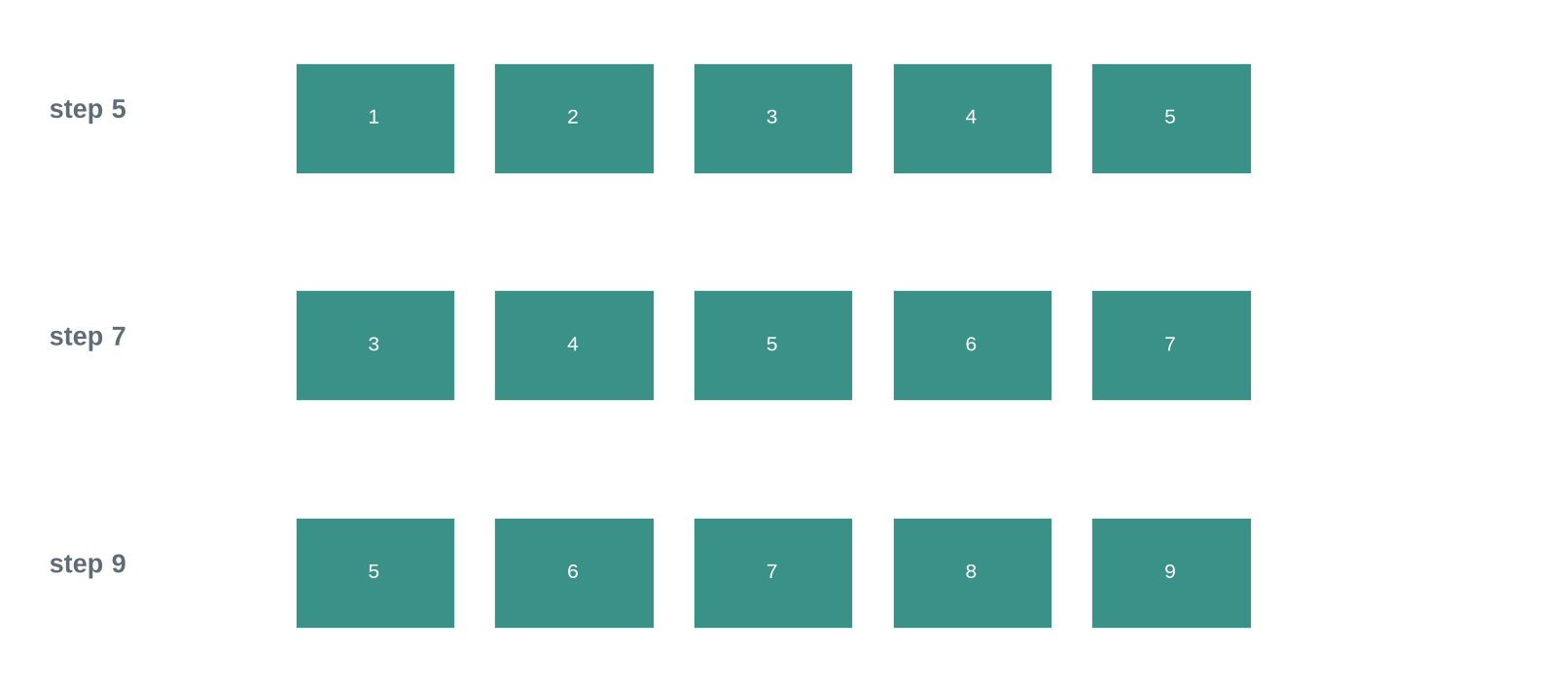
Long inputs can also conceal a simpler problem: the relevant evidence may be absent from the retained prefix. Sliding-window policies remove older tokens; fixed prompt templates may reserve too little output; and document conversion can add headings, markup, or duplicated material that consumes capacity. The input trace should retain token counts before and after formatting, the truncation decision, and the final token positions supplied to the model.

sequence=list(range(1,10)); limit=5
fig,axes=plt.subplots(3,1,figsize=(8.5,3.8))
for ax,end in zip(axes,[5,7,9]):
    window_tokens=sequence[max(0,end-limit):end]
    ax.axis("off"); ax.text(.02,.5,f"step {end}",weight="bold",color=grey,transform=ax.transAxes)
    for i,t in enumerate(window_tokens):
        x=.18+i*.13; ax.add_patch(Rectangle((x,.22),.105,.56,facecolor=teal,edgecolor="white")); ax.text(x+.052,.5,str(t),ha="center",va="center",color="white",fontsize=8)
plt.tight_layout(); plt.show()

Figure 28.5: A sliding-window policy retains recent tokens while discarding older positions once the configured context limit is reached.

The policy should distinguish discarded context from an intentional summary or retrieved representation. A summary is new model-generated text that may omit or distort facts. Retrieval is selected external evidence. Cached tokens are exact retained activations for previous IDs. These mechanisms can be combined, but their information properties differ and they should not be described by one generic claim of “memory”.

Serving constraints change the available context per request

At deployment, many requests may share accelerator memory. Each active sequence has a cache length, and a serving scheduler chooses batching, admission, eviction, and output limits. A context limit that fits one request can reduce concurrency or exceed memory under a busy workload. Conversely, aggressively capping prompts can improve latency while discarding evidence needed for a task. These are operating choices that should be measured against the task and service requirement.

cache_per_request_gib=1.0
available_gib=24
for active in [1,8,16,24]:
    print(active,"active requests require",active*cache_per_request_gib,"GiB of cache")

1 active requests require 1.0 GiB of cache
8 active requests require 8.0 GiB of cache
16 active requests require 16.0 GiB of cache
24 active requests require 24.0 GiB of cache

The calculation is deliberately incomplete because weights, temporary buffers, and allocator behaviour also occupy memory. It makes one relationship visible: higher concurrency, longer retained prefixes, and larger cache representations compete for the same hardware capacity. A serving result should specify whether its reported throughput is for isolated or concurrent requests, along with the prompt-length distribution.

Long-context errors require traces, not only accuracy totals

When a model misses evidence in a long prompt, a useful diagnostic records the original document, tokenised length, retained window, evidence span, retrieval or packing decision, generated tokens, and scoring rule. This can separate an error caused by truncation from one caused by poor retrieval, position sensitivity, or an incorrect answer despite available evidence. Aggregate accuracy remains useful, but it cannot make these failure modes distinguishable.

trace={"document_tokens":9100,"retained_tokens":8192,"evidence_position":7800,"truncated":False,"answer_correct":False}
print(trace)

{'document_tokens': 9100, 'retained_tokens': 8192, 'evidence_position': 7800, 'truncated': False, 'answer_correct': False}

Position and distraction controls should vary one feature at a time. For example, hold the question and answer constant while moving evidence from early to middle and late positions; then add unrelated material while keeping the evidence position fixed. These comparisons reveal whether a score changes with length, location, or competing content. They provide stronger evidence than a single long document with a single successful answer.

Length claims need tests that control position and distraction

A useful long-context evaluation places known evidence at several positions, asks a defined question, and compares performance across lengths and numbers of distractors. It should distinguish exact retrieval of a stated item from multi-step use of several items. Repeating a short fact many times, testing only the beginning of a prompt, or scoring a single favourable example cannot establish broad long-context use.

The evaluation should also record tokenizer, actual valid lengths, truncation and packing policy, prompt template, generation limit, sampling rule, and whether the answer was checked automatically or by people. Changing any of these can change the test. An answer that fails may reflect missing evidence, truncation, retrieval failure, cache error, decoding variation, or the model’s conditional distribution; the trace should make those possibilities distinguishable.

positions=[128,1024,4096,7168]
results={p:None for p in positions}
print("record evidence position and outcome:",results)

record evidence position and outcome: {128: None, 1024: None, 4096: None, 7168: None}

An inference record separates capacity from service quality

An inference report should include model and tokenizer version, context limit, maximum output length, prompt and output token distributions, prefill latency, decode latency or tokens per second, cache precision and layout, batch policy, hardware, concurrency, truncation behaviour, and failure policy. At least one cache-equivalence test and one boundary test at the configured maximum length should be retained.

The record supports operational decisions. It can show whether a system is limited by long-prompt prefill, by per-token decode latency, by memory available for concurrent caches, or by a context policy that discards needed evidence. A model card that says only “long context” cannot answer those questions.

inference_record={"context_limit":8192,"prompt_tokens":6200,"max_new_tokens":512,"prefill_ms":740,"decode_tokens_per_second":55,"cache_dtype":"float16"}
assert inference_record["prompt_tokens"]+inference_record["max_new_tokens"]<=inference_record["context_limit"]
print("length-budget check passed")

length-budget check passed

Common misconceptions

• A context limit is a guarantee of long-document reasoning. It specifies input capacity, not measured use of every position.
• Caching makes generation parallel. It removes repeated prefix computation but each selected token still conditions the next step.
• The cache stores the whole model state at no cost. It grows with layers, batch size, key-value heads, head width, and length.
• A document fits in context, so no truncation policy is needed. Prompt templates and reserved output also consume the total budget.
• Retrieval and a longer window solve the same problem. Retrieval selects evidence; a window determines available token capacity.

Exercises

1. Distinguish context length, prompt length, output length, and total length.
2. Calculate the available output budget for a stated maximum context and prompt.
3. Explain why prefill can run in parallel while decoding is sequential.
4. Derive the key-value cache element count for stated dimensions.
5. Estimate cache memory in bytes for float16 and float32.
6. Write a cache-equivalence test for a small causal model.
7. State one source of disagreement between cached and full-prefix decoding.
8. Compare the growth of dense prefill attention and cache storage with length.
9. Design a position-controlled long-context retrieval test.
10. Explain why a fact at the first position is an incomplete long-context test.
11. List metadata needed to interpret a tokens-per-second claim.
12. Describe a truncation policy for a prompt that exceeds the configured window.
13. Explain how grouped-query attention changes cache memory.
14. State why token count is not equivalent to a page count.
15. Separate a retrieval failure from a generation failure in an evaluation trace.
16. Identify the chapter that compares decoding and sampling policies.

Summary

Context windows define a finite token-level information boundary. Long prompts create prefill cost, and sequential generation requires one conditional decision after another. Key-value caches avoid repeated projection of earlier tokens but grow linearly with retained sequence length and must be tested against full-prefix decoding.

Capacity, retrieval, and demonstrated long-context use are distinct claims. Chapter 28 compares the policies that select tokens from a next-token distribution; Chapter 33 examines retrieval-augmented generation as a complete pipeline.

Looking ahead

The context window and cache determine which prefix the model can condition on and the cost of extending it. Chapter 28 examines the further policy that turns each next-token distribution into an emitted sequence.

Further reading

The original Transformer architecture and its attention cost are specified by Vaswani et al. (2017). FlashAttention describes an IO-aware exact attention implementation that changes practical memory behaviour without changing the attention result (Dao et al. 2022).

Dao, Tri, Daniel Y. Fu, Stefano Ermon, Atri Rudra, and Christopher Ré. 2022. “FlashAttention: Fast and Memory-Efficient Exact Attention with IO-Awareness.” Advances in Neural Information Processing Systems 35: 16344–59. https://arxiv.org/abs/2205.14135.

Vaswani, Ashish et al. 2017. “Attention Is All You Need.” Advances in Neural Information Processing Systems 30.